Difference between revisions of "Team:IISc-Bangalore/Model"
| Line 220: | Line 220: | ||
<h3>Electron microscopy</h3> | <h3>Electron microscopy</h3> | ||
| − | Multiple dilutions of pure gas vesicles suspended in PBS were imaged under a Scanning Electron Microscope after applying a 10nm gold sputter. In the images, gas vesicles can be seen as translucent polygon shaped particles. Note that some lysed gas vesicle membranes are also seen in the image owing to the drying step during the sample preparation that precedes electron microscopy. Air drying can be carried out over a longer period of time to reduce the number of such events. | + | Multiple dilutions of pure gas vesicles suspended in PBS were imaged under a Scanning Electron Microscope after applying a 10nm gold sputter. In the images, gas vesicles can be seen as translucent polygon shaped particles. Note that some lysed gas vesicle membranes are also seen in the image owing to the drying step during the sample preparation that precedes electron microscopy. Air drying can be carried out over a longer period of time to reduce the number of such events. Three dilutions were prepared for microscopy, out of these the 0.01ug/ul samples gave the best results. |
| + | |||
| − | |||
<img src="https://static.igem.org/mediawiki/2017/e/ea/T--IISc-Bangalore--Model-SEMWT1.png" width=400px> | <img src="https://static.igem.org/mediawiki/2017/e/ea/T--IISc-Bangalore--Model-SEMWT1.png" width=400px> | ||
<img src="https://static.igem.org/mediawiki/2017/5/54/T--IISc-Bangalore--Model-SEMWT2.png" width=400px> | <img src="https://static.igem.org/mediawiki/2017/5/54/T--IISc-Bangalore--Model-SEMWT2.png" width=400px> | ||
| + | |||
| + | Images 1 and 2: Gas vesicles at 40000x magnification under a SEM (0.01 ug/ul). | ||
Revision as of 13:24, 28 October 2017


| Sponsors | |||||
|---|---|---|---|---|---|
 |
 |
 |
|||
 |
 |
||||
| Contact | |||||
|---|---|---|---|---|---|
|
|
|
|||
Gas Vesicle Structure
Gas vesicles are proteineceous nano-structures that are utilized by many aquatic micro-organisms like halo-bacteria and some algae to provide buoyancy. The structure and arrangement is highly conserved between organisms with width being almost the only widely varying parameter. They contain gases which diffuse in during formation and are kept localised by the hydrophobicity of the inner membrane. Unlike true vesicles, these are made of proteins instead of phospholipids and are hence of considerable interest. Each gas vesicle is composed of two primary protein monomers, the gas vesicle forming proteins A (GvpA) and C (GvpC). The entire structure will be discussed in the following sections.
Verification of presence of Gas VesiclesThe easiest way to assay presence of gas vesicles is their disappearance under high pressure under a microscope. This was observed even during normal experiments. Fully filled micro-centrifuge tubes containing dilute gas vesicle suspensions lost their faint opalescence when the tube was closed (this did lead to a loss of samples). A more strict assay was done using DLS (See Dynamic Light Scattering) and SEM Imaging to pinpoint the exact size of the nano-particles. It was found that these gas vesicles have an effective hydrodynamic radius of around 230nm. This estimate was particularly valuable in the development of our model.
GvpA
The gas vesicle forming protein A (~8kDa) forms the main ribbed structure of the gas vesicle. The 3-Dimensional structural model of the protein was recently decoded by Strunk et.al ([1]). As was noted, the best probable docking pattern in a vesicle involves formation of a dimer and their consequent stacking. We intended to re-create the whole gas vesicle structure from this data and try to explain the growth pattern noticed during their formation. It is interesting to note that the hydrophobicity of the internally exposed part of GvpA is what keeps the gases from diffusing out.
GvpC
The gas vesicle forming protein C is the second most abundant protein found in the nanostructure. It is still far rarer compared to GvpA (1:25 molar ratio, [2]) and does not contribute to the structure but rather to the integrity of the gas vesicle. The vesicles used in the various experiments were stripped of GvpC before use and hence were much more sensitive compared to wild type gas vesicles. The critical pressure for the gas vesicles was found to reduce drastically on the removal of this protein.
Stacking of proteins in a GV nanoparticle
3-Dimensional structure of the nanoparticle
Effective buoyant density
Most of the physical properties of the gas vesicles were uncovered by Walsby et al. In their groundbreaking review ([3]). They calculated the average buoyant density of a gas vesicle to be around 120kgm-3. Note that while this density if much less than that of water, it doesn’t necessarily imply a flotation advantage due to the presence of diffusive forces in a suspension. The smaller the particle, higher is the magnitude of these diffusive interactions and more is the deviation from the ideal concentration profile in a column. The mathematical model part of our project deals with finding how these profiles evolve for overtime and how this evolution changes when we purposefully make them flocculate using agents like chitosan and biotin-streptavidin.
Mathematical Model
The following sections detail the development of our model which deals with the dynamics of gas vesicle motion in a medium and how their concentration profiles change over time.
Terminal Velocity
A floating particle in a media experiences multiple types of forces, some of which are more prominent than others. Given the buoyant density of the particle, we can find the terminal velocity by equating all the upward forces to the downward ones and solving for velocity from the stokes’ drag term.

Assuming the gas vesicle to be of the shape given above, its volume in terms of length l, half angle θ and radius r is given by,
\[ V = \pi r^{2}(l+\frac{2}{3}r cot \theta) \tag{1.1} \label{eq:1.1} \]So, the buoyant force on the gas vesicle is given by,
\[ F_b=V\rho g = \rho g\pi r^{2}(l+\frac{2}{3}r cot \theta) \tag{1.2} \label{eq:1.2} \]Where ρ is the density of the media.
Similarly, the force due to gravity is,
\[ F_w=V\rho_{gv} g = \rho_{gv} g\pi r^{2}(l+\frac{2}{3}r cot \theta) \tag{1.3} \label{eq:1.3} \]Where ρgv is the buoyant density of the gas vesicle.
When the particle reaches its terminal velocity, all the forces are balanced. Thus we can equate,
\[ F_{d} + F_{w} = F_{b} \tag{1.4} \label{eq:1.4} \]The viscous drag is usually a complex function of particle shape and size, in our case however, the DLS experiment directly gives the hydrodynamic radius of the particle. Hence we can use the well known expression for drag on a spherical particle given by,
\[ F_{d}=6\pi\eta R_{H} v \tag{1.5} \label{eq:1.5} \]Where vt is the terminal velocity and RH the hydrodynamic radius.
Solving for vt, we get
\[ v_{t}=\frac{Vg}{6\pi\eta R_H} (\rho-\rho_{gv}) \tag{1.6} \label{eq:1.6} \]The various parameters can be modified to find the terminal velocity for a particular kind of nanoparticle after measuring the hydrodynamic size with a DLS system. It is interesting to note that while the hydrodynamic radius is a linear function of the size of the gas vesicle, the volume scales as a cube of the radius. This leads to the logical deduction that the terminal velocity will increase if the particles are allowed to aggregate.
For a normal H. Salinarium gas vesicle, the terminal velocity comes out to be of the order of 10 nm/s . This is incredibly slow considering the size of a gas vesicle is an order of magnitude larger than this number.
Peclet number
The Peclet number is a dimensionless quantity that is used to determine the relative magnitudes of advective and diffusive transport phenomena. In the case of a particle undergoing flotation(or sedimentation), it can be easily calculated by taking the following ratio,
\[ P_e=\frac{Lu}{D} \tag{2.1} \label{eq:2.1} \]Where L is the characteristic length scale in the system (~200nm in the case of a gas vesicle), u the local velocity of the fluid and D the mass diffusion coefficient.
The Einstein relation for a spherical particle gives the Diffusion coefficient from the viscosity of the medium through the following relation,
\[ D=\frac{k_{b}T}{6\pi \eta R_{H}} \tag{2.2} \label{eq:2.2} \]Now, the terminal flow velocity from the last section can be used to calculate the Peclet number for this system. If the Peclet number is extremely small compared to 1, diffusion is dominant over advective transfer and must be considered during our calculations.
For a typical gas vesicle particle at room temperature (T = 273K),
L ~ 500nm
u ~ 10nm/s
RH ~ 200nm
Evolution of gas vesicle concentration profile in a column
Experimental Data
Visual Analysis
Flotation Spectrophotometry
Chitosan
Double replicates of four different concentrations of chitosan were used with gas vesicles (30ul stock) and the resulting solutions were diluted to 2ml to perform a flotation spectrophotometry assay.
| Tube Label | Effective gas vesicle concentration (ng/μl) |
Effective chitosan concentration (ng/μl) |
Remarks |
|---|---|---|---|
| 1 | 15 | 0 | Control tube |
| 2A | 15 | 5 | First replicate |
| 2B | 15 | 5 | Second replicate |
| 3A | 15 | 50 | First replicate |
| 3B | 15 | 50 | Second replicate |
| 4A | 15 | 500 | First replicate |
| 4B | 15 | 500 | Second replicate |
| 5A | 15 | 5000 | First replicate |
| 5B | 15 | 5000 | Second replicate |
The data from the spectrophotometer assays for chitosan can be found here.
An analysis of the data is given in the results section
Electron microscopy
Multiple dilutions of pure gas vesicles suspended in PBS were imaged under a Scanning Electron Microscope after applying a 10nm gold sputter. In the images, gas vesicles can be seen as translucent polygon shaped particles. Note that some lysed gas vesicle membranes are also seen in the image owing to the drying step during the sample preparation that precedes electron microscopy. Air drying can be carried out over a longer period of time to reduce the number of such events. Three dilutions were prepared for microscopy, out of these the 0.01ug/ul samples gave the best results.
 Images 1 and 2: Gas vesicles at 40000x magnification under a SEM (0.01 ug/ul).
Dynamic Light Scattering
Gas vesicle suspensions prepared as in the spectrophotometry assay were used to perform Dynamic light scattering. Three replicates of each concentration were run through the machine thrice. It was noted that the average particle size decreased after every run indicating the particles were either sedimenting or floating up.
The data can be accessed here.
Results
Chitosan
The data when averaged over the replicates shows a marked faster decrease in OD as time passes for chitosan treated gas vesicles. The gas vesicles without chitosan show no significant decrease over a duration of two hours while the ones with the maximum chitosan concentration show a fast decrease at the start which saturates as time passes. All other curves lie in an intermediate region(Fig 1). At very high concentrations, it was seen that the saturation point shifted upwards. We postulate this is because of the gas vesicles were irreversibly denatured by the action of excessive acetic acid concentration during chitosan incubation. More detailed analysis can be conducted to find the optimum concentration at which maximum flotation is achieved. The plot was smoothed out over a window of 85 data points giving the smooth profiles. (Fig 2)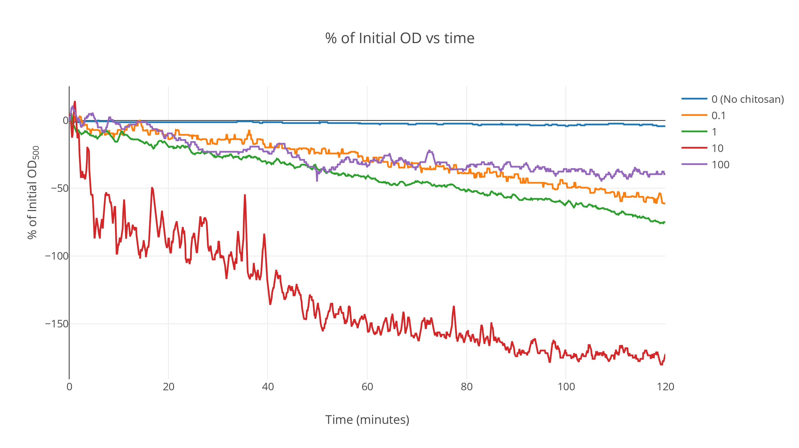

It was found that the particle size increased considerably on addition of chitosan. The data from the Dynamic light scattering experiment is plotted in Figure 3. The points were fit to a quadratic curve.
