Team:Peking/Model
Overview
Background
In our design, after having designed the flip flop, the device can remember the information of its state, the next step is to transform the state into an actual function. To achieve this transformation, we first needed a “reader” to read out the current state. At this point the control unit comes into play. A control unit is a DNA sequence with recombinase sites whose expression is controlled by recom-binase and RDF by reversing or deleting a promoter and/or a terminator. To make the control unit reliable and predictable, we first need to be able to predict the behaviors of its “building blocks” (or “elements” in electrical engineering), from which we weave our engineer’s perspective into the biolog-ical system. However, we need to make some adaptations and adjustments to these “elements” to make them usable.Controller
Intention of the Model
In this model, we aim to describe the sequence modification process of the control unit sequence with recombination sites. Different recombinases are expressed in series to alter the direction of terminators between corresponding recombination sites on the control unit circuit. The combination of unidirectional terminators in different directions (reverse or foward) determines the state of RNA polymerase flux, thus controlling expression of the downstream gene.
Though we have done simulation of recombinase dynamics in the previous section, it is necessary to consider two key concepts of biological processes: 1. population behavior 2. stochastic process
The reason for modeling cell population behavior is that deployment of synthetic bacterial devices would certainly involve populations of cells. Furthermore, we demonstrate our design through continuous imaging of entire cell cultures. This is a theory-experiment interaction procedure. The reason for stochastic modeling is self-evident. Cellular biological processes, especially gene expression, are innately noisy and stochastic.[^Footnote1] Previous work has demonstrated the effectiveness of the integration of population-level dynamics and stochastic cellular responses to inputs.[^Footnote2]It is important to explain how stochastic single-cell responses affect overall population-level distributions and behavior.
This section describes a Markov model of recombinase-based DNA flipping and a Gillespie stochastic simulation method[^Footnote3] to observe theoretical sequence state evolution. We will focus on our demonstration design, which can be generalized to other designs.
Biological Basis
The control units are implemented experimentally by transforming a plasmid into an E. coli. This plasmid has similar structure as the reporter plasmid in the previous section. However, in this situation the sequence fragments being inverted are terminators. Using experimentally screened uni-directional terminators, the transcription or polymerase flux4 can be precisely controlled. The figure below illustrates the result of the design software. (超链接到software)
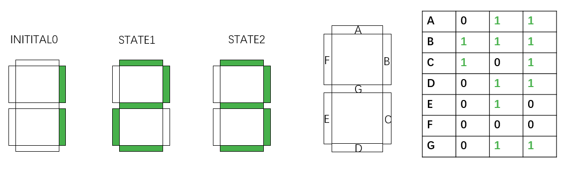
In the seven-segment decoder tube demonstration, if we would like to display “1-2-3” counting, 3 kinds of control units have to be transformed into 3 strains of bacteria. 2 of them has only one pair of recombination sites, and only undergoes recombinase inversion once. The other one has two nested recombination sites. Successive inversion results in the same state as the initial one.
Model Composition and Assumptions
A Markov process is defined upon a specific state space. We define that each state occupies a specific state. Then we can use Markov models to track cell state changes over time. This “state” consists of two parts: the state of recombination sites on the control unit sequence and the concentration or molecule number of two types of recombinases A and B. This definition was first proposed by Victoria Hsiao and colleagues to model a population-based event detector.5 The state of a single cell is defined by the DNA state and the copy numbers of integrases A and B. We denote the state of a single cell by (DNA, IntA, IntB).
Cell States
All of the four possible DNA states are: the initial state (\(S_{init}\)), the IntA inversion only state (\(S_a\)), the IntB inversion only state (\(S_b\)), and the IntA then IntB inversion state (\(S_{ab}\)). We omit the state IntB then IntA inversion state (\(S_{ba}\)) because in our design and experiments, integrase expression is always induced in order. IntB expression can never be triggered before that of IntA. These states and transitions by recombinase inversions are illustrated below.Our implementation requires that the control unit sequence on a stringent, low copy number plasmid. Thus we assume that each cell only has one copy of the control unit. Uni-directional terminators are screened by the criterion that the forward terminator strength[^Footnote6] exceeds the reverse one by a few orders of magnitude. This allows us to assume that when the terminator is in the forward direction, it can completely block RNA polymerase, while in the reverse direction, it cannot function.(此处有链接到terminator实验页面)
Integrase Production and Tetramerization
Serine integrases are produced as monomers that form dimers, search for specific attB and attP sequences, and, once both attB and attP sites are occupied, form a tetramer (dimer of dimers) that digests, flips and re-ligates the DNA[^Footnote7]. In this model we also consider leaky expression of the recombinases, because of observation of such phenomena in recombinase characterization experiments. Furthermore, induction of recombinase expression happens in order and we assume that at each time point, only one of the two inducers (a and b) exists. Thus we define the following table of state transitions and parameters: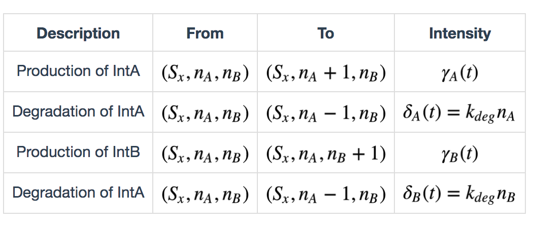
\(x \in \{init, a, b, ab\})\), \(\gamma_A(t)\) and \(\gamma_B(t)\) are defined as follows: \[ \gamma_A(t) = \begin{cases} k_{prodA} + k_{leakA}, & \text{if inducer a exists} \\ k_{leakB}, & \text{otherwise} \end{cases} \] \[ \gamma_B(t) = \begin{cases} k_{prodB} + k_{leakB}, & \text{if inducer a exists} \\ k_{leakB}, & \text{otherwise} \end{cases} \]
The serine integrases need to tetramerize prior to DNA recombination. Each DNA binding site (attB and attP) is bound by two copies of integrase monomers in an independent manner to form a dimer. Once both of the binding sites on both DNA attachment sites are occupied, a dimer of the dimers (tetramer) is formed and recombination can occur. Here we deduce the reaction propensity of the tetramerization process. We only focus on the number of integrase molecules inside the cell, and ignore the detailed process of transcription and translation, and represent the process with a single parameter.
\(S_x:Int_i (i = 1,2,3,4) (x \in \{init, a, b, ab\})\) denote the DNA-integrase complexes where \(i\) denote the number of integrase molecules bound to DNA sequence. DNA recombination occurs when the complex state is at \(S_x:Int_4\), which means the tetramerization of integrases on the DNA. Because of independent binding of DNA sequence with integrase dimers, the transition of states can be modeled by the following equations: \[ S_x \rightleftarrows S_x:Int_1 \rightleftarrows S_x:Int_2 \rightleftarrows S_x:Int_3 \rightleftarrows S_x:Int_4 \]
where the binding rate of DNA recombination sites (attB, attP) and integrase dimers is \(k_{bind}\) (reaction from left to right side) and unbinding rate is \(k_{unbind}\). The dynamics can be modeled by the following ordinary differential equations. \(\mathbb{P}_t(S_x:Int_i, n_*) (* = A, B)\) is the joint probability distribution.
\[
\frac{d}{dt}\mathbb{P}_t(S_x, n_*) = -k_{bind}n_*\mathbb{P}_t(S_x, n_*) + k_{unbind}\mathbb{P}_t(S_x:Int_1, n_*)
\] \[
\frac{d}{dt}\mathbb{P}_t(S_x:Int_1, n_*-1) = -(k_{bind}(n_*-1)+k_{unbind})\mathbb{P}_t(S_x:Int_1, n_*-1) + k_{bind}n_*\mathbb{P}_t(S_x, n_*) + k_{unbind}\mathbb{P}_t(S_x:Int_2,n_*-2)
\] \[
\frac{d}{dt}\mathbb{P}_t(S_x:Int_2, n_*-2) = -(k_{bind}(n_*-2)+k_{unbind})\mathbb{P}_t(S_x:Int_2, n_*-2) + k_{bind}(n_*-1)\mathbb{P}_t(S_x:Int_1, n_*-1) + k_{unbind}\mathbb{P}_t(S_x:Int_3,n_*-3)
\] \[
\frac{d}{dt}\mathbb{P}_t(S_x:Int_1, n_*-3) = -(k_{bind}(n_*-3)+k_{unbind})\mathbb{P}_t(S_x:Int_3, n_*-3) + k_{bind}(n_*-2)\mathbb{P}_t(S_x:Int_2, n_*-2) + k_{unbind}\mathbb{P}_t(S_x:Int_4,n_*-4)
\] \[
\frac{d}{dt}\mathbb{P}_t(S_x:Int_4, n_*-4) = -k_{unbind}n_*\mathbb{P}_t(S_x:Int_4, n_*-4) + k_{bind}(n_*-3)\mathbb{P}_t(S_x:Int_3, n_*-3)
\]
We assume that binding and unbinding of integrase molecules to DNA equilibrate fast enough compared to the dynamics of DNA recombination, and the production and degradation of integrases (See Parameter Supplemental) and hence the above equations converge to an equilibrium while \(n_*\) remain constant (equilibrium approximation). Let the above equations all equal to zero and solve in terms of \(\frac{d}{dt}\mathbb{P}_t(S_x:Int_4, n_*-4)\), we can write:
\[ \frac{d}{dt}\mathbb{P}_t(S_x:Int_4, n_*-4) = \frac{n_* (n_*-1)(n_*-2) (n_*-3)}{K_{d*}^4 + K_{d*}^3 n_* + K_{d*}^2 n_* (n_*-1) + K_{d*}n_*(n_*-1)(n_*-2) + n_* (n_*-1)(n_*-2)(n_*-3)} \] (\(K_{d*} = k_{unbind}/k_{bind}\))
Continuous-time Markov Process
Rather than accounting fro all individual DNA-integrase interactions, we have created a minimal model of stochastic transitions. Here only the final DNA states \((S_o, S_a, S_b, S_{ab})\) and the number of integrase monomer molecules (IntA, IntB) are tracked and all integrase activity is encompassed in the \(k_{flip*} (*=A,B)\) term. Because no cooperativity has been observed in Bxb1 or TP901-1 DNA binding, e.g. occupation of attB does not increase the probability of attP binding, we assume that the flipping activity is zero unless at least four molecules are present. Then, the propensity function for state transitions is a function of integrase concentration (equivalent to protein molecule number in cell, if cell volume is assumed to be constant):\[ \alpha_i(Int_*) = k_{flip*}(\frac{n_* (n_*-1)(n_*-2) (n_*-3)}{K_{d*}^4 + K_{d*}^3 n_* + K_{d*}^2 n_* (n_*-1) + K_{d*}n_*(n_*-1)(n_*-2) + n_* (n_*-1)(n_*-2)(n_*-3)}) \] \(i = 1, 2, 3; * = A, B\)
Then the table of state transition and intensities can be completed. We consider three kinds of state transitions as described previously: \(S_{init}\) to \(S_a\), \(S_{init}\) to \(S_b\), and \(S_a\) to \(S_{ab}\). \(S_{init}\) to \(S_b\) is due to missing of integrase A flipping. This transition denotes the system’s ineffective fraction.
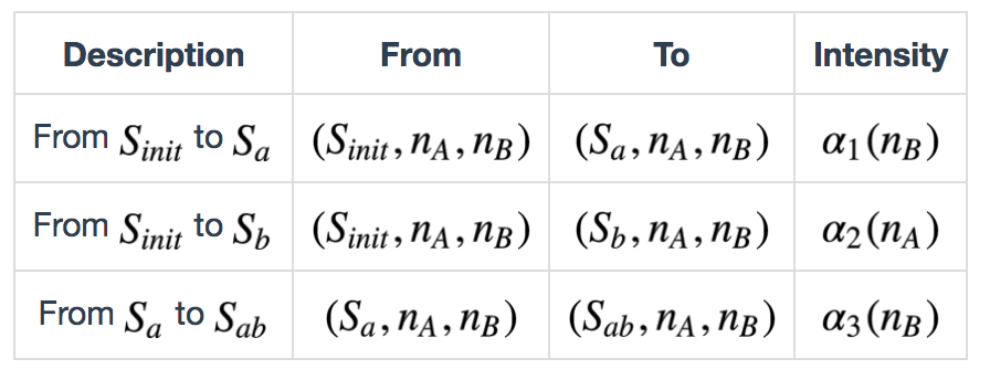
Numbers of cells occupying each state are calculated by the summing equation below: span class="math display">\[ S_{i} = \sum_{n_A=0}^{\infty}\sum_{n_B=0}^{\infty} S(i,n_A,n_B), i \in \{S_{init},S_a,S_b\} \] because we only concentrate on the cell numbers, not the specific protein copy numbers in cells.
Simulation Results
Simulation Setting
In the simulation in this section, we consider induction with step inputs, where the inducers are either present or not present. Concentrations of the inducers when they are ‘’on’’ will be held constant. Also, it is important to note that inducer \(a\) is still present during and after time \(\Delta t\) when inducer \(b\) is introduced. We predict qualitative circuit behavior with biologically plausible parameters simplified to a minimal set: integrase production, degradation, tetramerization and DNA flipping. The integrase monomer dissociation constant \(K_{d*} (*=intA, intB)\) was estimated from Singh’s work. For more details of parameter setting for simulation please see our supplement page.Whole Process and Analysis: Guidance for experimentalists
Qualitative prediction of the population behavior of 3000 or 1000 cells was simulated. We first limit the simulator to the situation of only one pair of recombination sites on the circuit. From the results below we can see that after approximately 10h the recombinase intA complete the flipping and the reaction is rather efficient.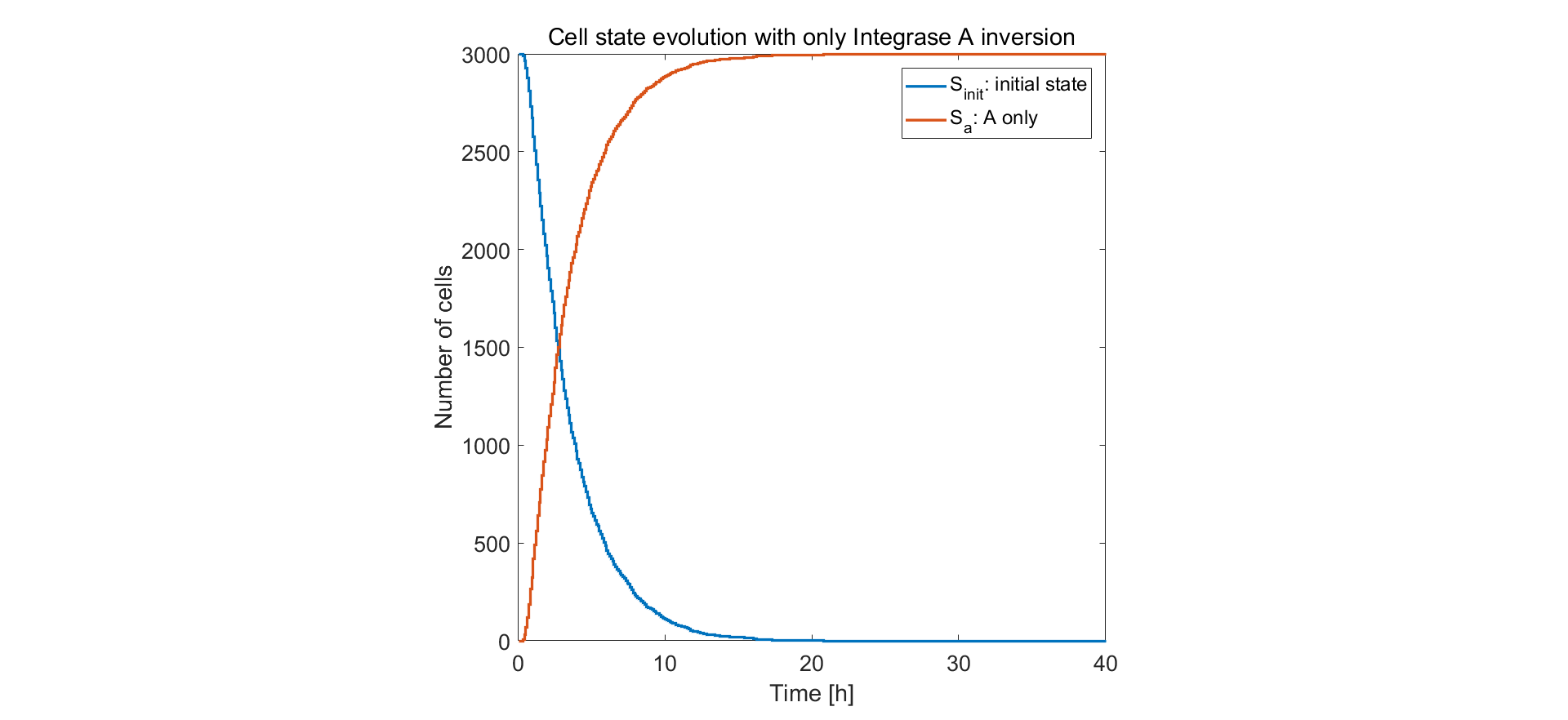
Fig.1. Simulation result of only one pair of recombination sites on control unit circuit
The results for two pairs of recombination sites are shown below. We did two simulations. The first one (shown in the left figure), with two recombinases induced with no time separation, the system acts in an unsatisfactory way and approximately half of the cells are in the undesired state \(S_b\). In the second one, inducing of intA and intB are separated with 5 hours. Then the system performs rather stably, with approximately 90% cells in desired state. This provides guidance for team members working in the lab.
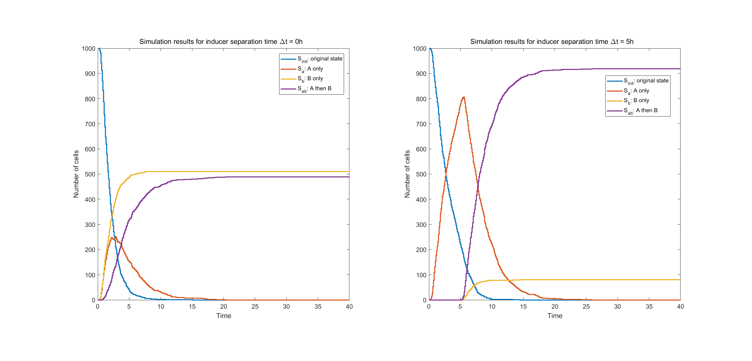
Fig.2. Simulation result of two pairs of recombination sites
The left figure shows state evolution with no time separation in inducing events A and B. The right figure shows state evolution with time separation of \(\Delta t = 5h\).
Finally we show specific cell transitions in Gillespie simulation. 100 cells are sampled from the population. Each vertical line denotes a cell state transition event (from \(S_{init}\) to \(S_a\), \(S_{init}\) to \(S_b\), from \(S_a\) to \(S_{ab}\)). The last two subplots show the simulation results of protein expression in single cell.
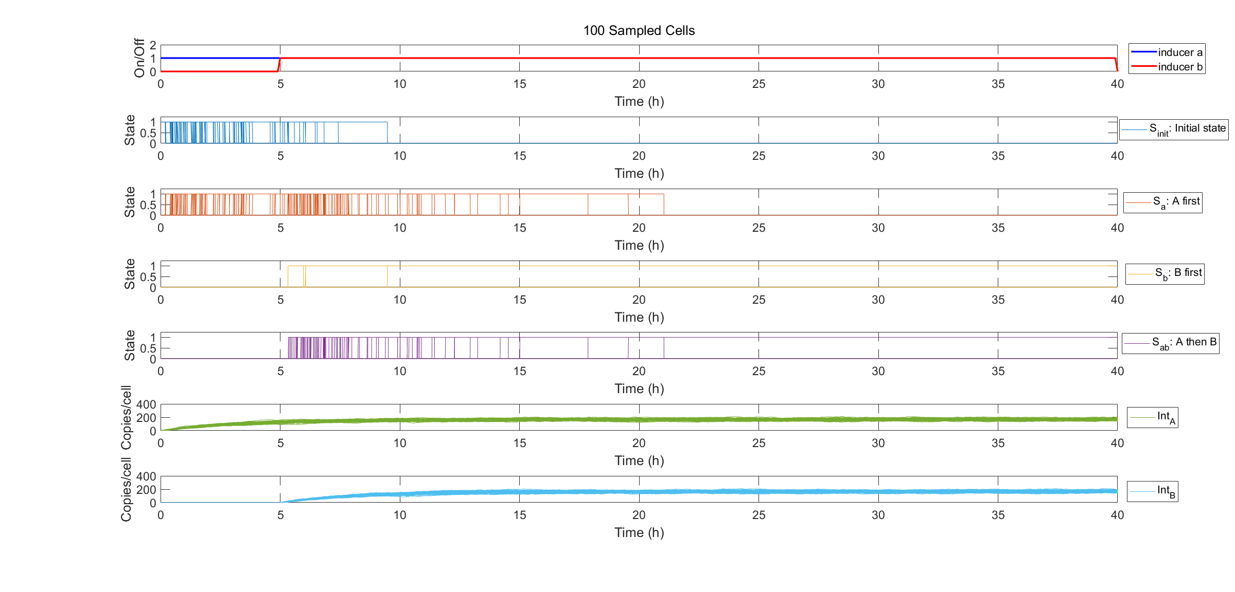
Fig.3. Specification of state transitions in Gillespie simulation using 100 sampled cells.
Clock
Intention of the Model
We attempts to develop a framework of biological sequential circuits that are programmable. The envisioned circuit is capable of both storing states in DNA and automatically running a series of instructions in a specific order. According to our design, our bio-flip-flop has two promoters, each triggered by an inducing signal. Therefore, if we would like to build an automatic triggering system for the bio-flip-flop, we need at least two signals in our clock. It is then self-evident to incorporate the classic structure in synthetic biology: the repressilator.
This model serves as a proof of concept for such implementation. We first constructed an ordinary differential equation (ODE) system to describe the repressilator, then we used two repressor proteins expressed by the repressilator to regulate the two promoters. Finally we adjusted parameters and gave a simulation result as a proof of the possibility of repressilator-driven bio-flip-flop.
Biological Basis and Assumptions
The repressilator is a synthetic genetic regulatory network consisting of a ring-oscillator with three genes, each expressing a protein that represses the next gene in the loop.[^Footnote1] This network was designed from scratch to exhibit a stable oscillation which is reported via the expression of green fluorescent protein, and hence acts like an electrical oscillator system with fixed time periods. The repressilator consists of three genes connected in a feedback loop, such that each gene represses the next gene in the loop, and is repressed by the previous gene.
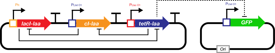
Fig.1. The genetic structure of the repressilator network
We decided to implement our repressilator-triggered bio-flip-flop with two repressor proteins regulating the two promoters’ transcription. The basis of ODE system construction is illustrated as follows:
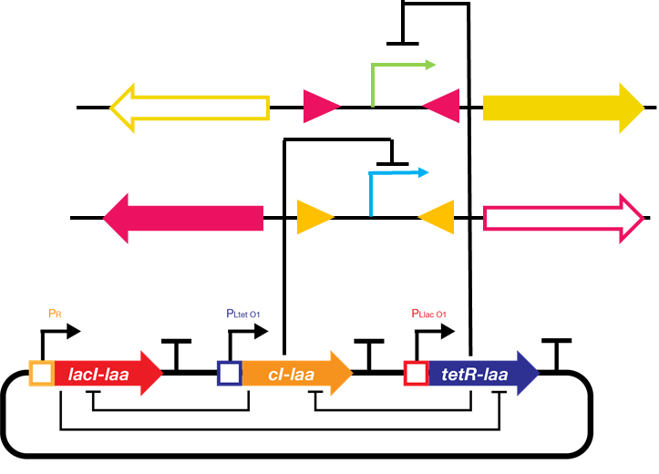
Fig.2. Schematic drawing of the repressilator-driven bio-flip-flop
The upper promoter (X) is \(P_{LtetO}\) and is repressed by tetR protein. The lower promoter (Y) is \(P_{R}\) and is repressed by cI protein.Simulation of bio-flip-flop starts at a later time than repressilator because the expression levels of the repressor proteins at the beginning is not high enough.
Equations and Parameters
Repressilator
The following table lists the reactions in the repressilator network. X, Y, Z represent LacI, TetR and cI mRNAs, and PX, PY, PZ represent the corresponding proteins.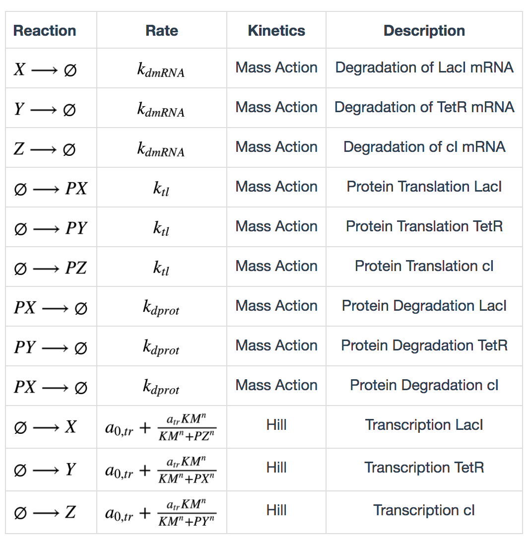
Calculation of degradation rates are described as follows: \[ k_{dmRNA} = \frac{ln(2)}{\tau_{mRNA}} \] \[ k_{dprot} = \frac{ln(2)}{\tau_{protein}} \] \(\tau_{mRNA}\) and \(\tau_{protein}\) are half lives of mRNA and protein. Calculation of maximum transcription rate: \[ a_{tr} = 60(ps_a - ps_0) \] \(ps_a\) is “tps active” and \(ps_0\) is “tps_repressive”. Calculation of translation rate: \[ k_{tl} = \frac{eff}{t_{ave}} \] \(eff\) is translation efficiency and \(t_{ave}\) is average mRNA life time. \(t_{ave} = \frac{\tau_{mRNA}}{ln(2)}\)
Transcription in bio-flip-flop
The transcription kinetics in the bio-flip-flop were modified to be repressed by repressors. These can be described by the following equations: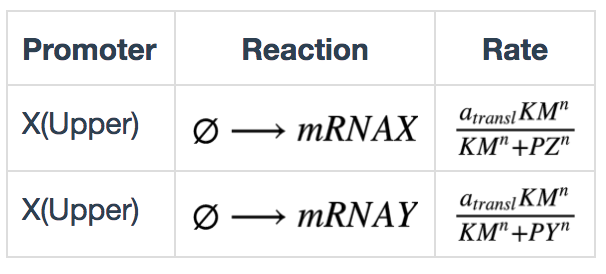
Simulation Results
We conducted our simulation using Tellurium[^Footnote3], a Python-based simulation platform. We first adjusted the parameters protein half life and mRNA half life (equivalently transcription and translation of repressor proteins) to adjust oscillation period as the one observed in the experiment. (此处链接到clock实验)
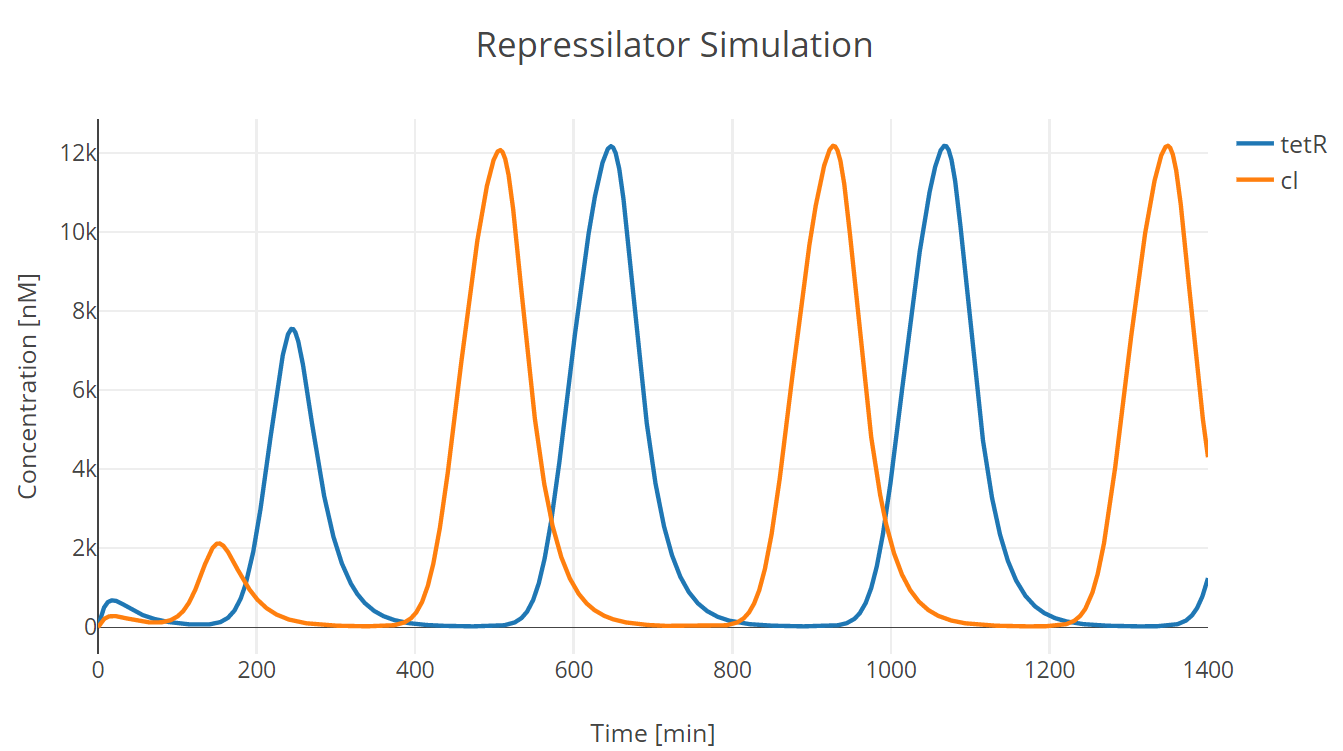
Fig.1. Repressilator simulation results of tetR and cI protein
Then we incorporate the bio-flip-flop into the model, and we got the following simulation results:
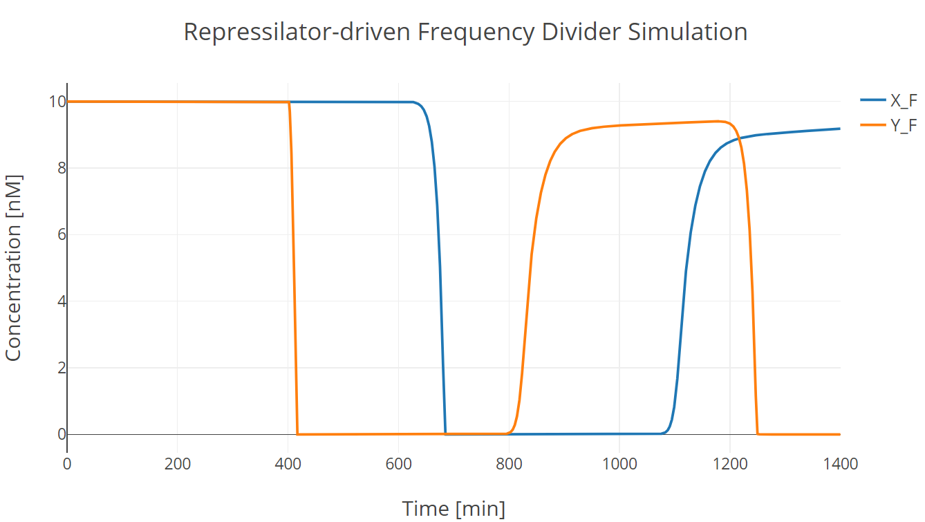
Fig.2. Repressilator-driven frequency divider simulation with two trigger signal groups
X_F and Y_F have the same meaning as those described in Recombinase section. (此处有超链接到第一个model子页面)
In this simulation experiment, the flip-flop lost approximately 10% of its initial state after two trigger signal groups.