Difference between revisions of "Team:NTHU Taiwan/Model"
| (39 intermediate revisions by 8 users not shown) | |||
| Line 20: | Line 20: | ||
display:block; | display:block; | ||
float:left; | float:left; | ||
| − | font-family:' | + | font-family: 'Helvetica', sans-serif; |
background-color: #F6F6E3; | background-color: #F6F6E3; | ||
} | } | ||
| Line 39: | Line 39: | ||
.igem_2017_content_wrapper h1, .igem_2017_content_wrapper h2 .igem_2017_content_wrapper h3, .igem_2017_content_wrapper h4, .igem_2017_content_wrapper h5, .igem_2017_content_wrapper h6 { | .igem_2017_content_wrapper h1, .igem_2017_content_wrapper h2 .igem_2017_content_wrapper h3, .igem_2017_content_wrapper h4, .igem_2017_content_wrapper h5, .igem_2017_content_wrapper h6 { | ||
| + | font-family: Helvetica; | ||
padding: 50px 0px 15px 0px; | padding: 50px 0px 15px 0px; | ||
border-bottom: 0px; | border-bottom: 0px; | ||
| Line 45: | Line 46: | ||
} | } | ||
| + | |||
.igem_2017_content_wrapper .content { | .igem_2017_content_wrapper .content { | ||
| Line 52: | Line 54: | ||
.igem_2017_content_wrapper .content p{ | .igem_2017_content_wrapper .content p{ | ||
| + | font-family: Helvetica; | ||
color: #2C2C2C; | color: #2C2C2C; | ||
font-size: 1.4em; | font-size: 1.4em; | ||
| Line 59: | Line 62: | ||
text-justify:inter-ideograph; | text-justify:inter-ideograph; | ||
} | } | ||
| + | |||
.igem_2017_content_wrapper .content img{ | .igem_2017_content_wrapper .content img{ | ||
| Line 104: | Line 108: | ||
<!-- start of content --> | <!-- start of content --> | ||
<div class="igem_2017_content_wrapper"> | <div class="igem_2017_content_wrapper"> | ||
| + | <img width="25%" src="https://static.igem.org/mediawiki/2017/3/3d/T--NTHU_Taiwan--Project--gear.png"> | ||
<div style="text-align: center"> | <div style="text-align: center"> | ||
<h1 style="color:#DF6A6A">Model | <h1 style="color:#DF6A6A">Model | ||
| Line 112: | Line 117: | ||
<div class="content"> | <div class="content"> | ||
| + | <table style="line-height:27px;""border:3px #cccccc solid;" cellpadding="10" border='1';"font-size:25px;text-align:justify; | ||
| + | text-justify:inter-ideograph;";"line-height:30px> | ||
| + | <tr> | ||
| + | <td style="background-color: #f6f6e3;"text-align:justify; | ||
| + | text-justify:inter-ideograph;";"line-height:30px><center><h1>Overview</h1></center><br> | ||
| + | <font size=5> | ||
| + | 1. Conducted Simulation in order to simulate filter’s working ability and improve our design.<br><br> | ||
| + | 2. Used the equation of Michaelis-Menten kinetics model to test our HRP degradation efficiency.<br><br> | ||
| + | 3. Derived Freundlich Adsorption Isotherm model to measure the adsorption capacity of our filter.<br><br> | ||
| + | 4. Modeled the design life of our filter to predict the frequency of replacement of inner activated carbons.<br><br> | ||
| + | |||
| + | </font> | ||
| + | |||
| + | </td> | ||
| + | </tr> | ||
| + | </table> | ||
| − | <center>< | + | <center><h1> |
| − | + | Model 1: Enzyme kinetics | |
| − | </ | + | </h1></center><br><br><br> |
<p> | <p> | ||
| Line 134: | Line 155: | ||
<p> | <p> | ||
| − | The initial collision of E and S is a bimolecular reaction with the second-order rate | + | The initial collision of E (Enzyme) and S (Substrate) is a bimolecular reaction with the second-order rate |
| − | constant | + | constant k<sub>1</sub>. The ES complex can then undergo one of two possible reactions: k<sub>2</sub> is the first-order rate constant for the conversion of ES to E and P, and k<sub>-1</sub> is the first-order rate constant for the conversion of ES back to E and S.We assume that the formation of product from ES (the step described by k<sub>2</sub>) does not occur in reverse. |
</p> | </p> | ||
| Line 156: | Line 177: | ||
<p> | <p> | ||
| − | To simplify our analysis, we choose experimental conditions such that the substrate | + | To simplify our analysis, we choose experimental conditions such that the substrate concentration is much greater than the enzyme concentration and ES remains constant until nearly all the substrate has been converted to product. |
| − | + | ||
</p> | </p> | ||
| Line 255: | Line 275: | ||
</p> | </p> | ||
| − | < | + | |
| − | + | <h2> | |
The degradation rate under different EDCs concentration | The degradation rate under different EDCs concentration | ||
| − | + | </h2> | |
| − | </ | + | |
| Line 296: | Line 315: | ||
<p> | <p> | ||
| − | <img width="90%"src="https://static.igem.org/mediawiki/ | + | <img width="90%"src="https://static.igem.org/mediawiki/2017/e/eb/T--NTHU_Taiwan--Model--speed_degradation_62_EDC_concentration.png"> |
</p> | </p> | ||
| Line 306: | Line 325: | ||
<p> | <p> | ||
| − | <img width="90%"src="https://static.igem.org/mediawiki/2017/ | + | <img width="90%"src="https://static.igem.org/mediawiki/2017/3/34/T--NTHU_Taiwan--Model--speed_degradation_72_EDC_concentration.png"> |
</p> | </p> | ||
| Line 315: | Line 334: | ||
<p> | <p> | ||
| − | <img width="90%"src="https://static.igem.org/mediawiki/2017/ | + | <img width="90%"src="https://static.igem.org/mediawiki/2017/b/b6/T--NTHU_Taiwan--Model--speed_degradation_82_EDC_concentration.png"> |
</p> | </p> | ||
| Line 323: | Line 342: | ||
<p> | <p> | ||
| − | <img width="90%"src="https://static.igem.org/mediawiki/2017/ | + | <img width="90%"src="https://static.igem.org/mediawiki/2017/6/6c/T--NTHU_Taiwan--Model--speed_degradation_92_EDC_concentration.png"> |
</p> | </p> | ||
<p><center><font size=2> | <p><center><font size=2> | ||
Figure 4. degradation speed vs EDCs concentration under the maxmium EDCs concentration of 10^(-9) mg/L | Figure 4. degradation speed vs EDCs concentration under the maxmium EDCs concentration of 10^(-9) mg/L | ||
| − | </font></center></p> | + | </font></center></p><br><br><br> |
| Line 349: | Line 368: | ||
<p> | <p> | ||
| − | <img width="90%"src="https://static.igem.org/mediawiki/2017/ | + | <img width="90%"src="https://static.igem.org/mediawiki/2017/a/a7/T--NTHU_Taiwan--Model--T--NTHU_Taiwan--Model--50_degradation_62_EDC_concentration.png"> |
</p> | </p> | ||
| Line 357: | Line 376: | ||
<p> | <p> | ||
| − | <img width="90%"src="https://static.igem.org/mediawiki/2017/ | + | <img width="90%"src="https://static.igem.org/mediawiki/2017/0/06/T--NTHU_Taiwan--Model--T--NTHU_Taiwan--Model--50_degradation_72_EDC_concentration.png"> |
</p> | </p> | ||
| Line 365: | Line 384: | ||
<p> | <p> | ||
| − | <img width="90%"src="https://static.igem.org/mediawiki/2017/ | + | <img width="90%"src="https://static.igem.org/mediawiki/2017/8/8d/T--NTHU_Taiwan--Model--T--NTHU_Taiwan--Model--50_degradation_82_EDC_concentration.png"> |
</p> | </p> | ||
| Line 373: | Line 392: | ||
<p> | <p> | ||
| − | <img width="90%"src="https://static.igem.org/mediawiki/2017/ | + | <img width="90%"src="https://static.igem.org/mediawiki/2017/5/5e/T--NTHU_Taiwan--Model--T--NTHU_Taiwan--Model--50_degradation_92_EDC_concentration.png"> |
</p> | </p> | ||
| Line 381: | Line 400: | ||
<p> | <p> | ||
| − | <img width="90%"src="https://static.igem.org/mediawiki/2017/ | + | <img width="90%"src="https://static.igem.org/mediawiki/2017/f/f1/T--NTHU_Taiwan--Model--T_of_50_Degradation_Rate_12_EDC_saturation_point.png"> |
</p> | </p> | ||
| Line 389: | Line 408: | ||
<p> | <p> | ||
| − | <img width="90%"src="https://static.igem.org/mediawiki/2017/ | + | <img width="90%"src="https://static.igem.org/mediawiki/2017/2/27/T--NTHU_Taiwan--Model--75_degradation_61_EDC_concentration.png"> |
</p> | </p> | ||
| Line 397: | Line 416: | ||
<p> | <p> | ||
| − | <img width="90%"src="https://static.igem.org/mediawiki/2017/1/ | + | <img width="90%"src="https://static.igem.org/mediawiki/2017/1/1b/T--NTHU_Taiwan--Model--75_degradation_72_EDC_concentration.png"> |
</p> | </p> | ||
| Line 405: | Line 424: | ||
<p> | <p> | ||
| − | <img width="90%"src="https://static.igem.org/mediawiki/2017/ | + | <img width="90%"src="https://static.igem.org/mediawiki/2017/e/e4/T--NTHU_Taiwan--Model--75_degradation_82_EDC_concentration.png"> |
</p> | </p> | ||
| Line 413: | Line 432: | ||
<p> | <p> | ||
| − | <img width="90%"src="https://static.igem.org/mediawiki/2017/ | + | <img width="90%"src="https://static.igem.org/mediawiki/2017/4/4e/T--NTHU_Taiwan--Model--75_degradation_92_EDC_concentration.png"> |
</p> | </p> | ||
| Line 421: | Line 440: | ||
<p> | <p> | ||
| − | <img width="90%"src="https://static.igem.org/mediawiki/2017/9/ | + | <img width="90%"src="https://static.igem.org/mediawiki/2017/9/97/T--NTHU_Taiwan--Model--T_of_75_Degradation_Rate_12_EDC_saturation_point.png"> |
</p> | </p> | ||
| Line 429: | Line 448: | ||
<p> | <p> | ||
| − | <img width="90%"src="https://static.igem.org/mediawiki/2017/ | + | <img width="90%"src="https://static.igem.org/mediawiki/2017/3/38/T--NTHU_Taiwan--Model--95_degradation_62_EDC_concentration.png"> |
</p> | </p> | ||
| Line 437: | Line 456: | ||
<p> | <p> | ||
| − | <img width="90%"src="https://static.igem.org/mediawiki/2017/ | + | <img width="90%"src="https://static.igem.org/mediawiki/2017/3/39/T--NTHU_Taiwan--Model--95_degradation_72_EDC_concentration.png"> |
</p> | </p> | ||
| Line 445: | Line 464: | ||
<p> | <p> | ||
| − | <img width="90%"src="https://static.igem.org/mediawiki/2017/ | + | <img width="90%"src="https://static.igem.org/mediawiki/2017/8/8f/T--NTHU_Taiwan--Model--95_degradation_82_EDC_concentration.png"> |
</p> | </p> | ||
| Line 453: | Line 472: | ||
<p> | <p> | ||
| − | <img width="90%"src="https://static.igem.org/mediawiki/2017/ | + | <img width="90%"src="https://static.igem.org/mediawiki/2017/c/c0/T--NTHU_Taiwan--Model--95_degradation_92_EDC_concentration.png"> |
</p> | </p> | ||
| Line 461: | Line 480: | ||
<p> | <p> | ||
| − | <img width="90%"src="https://static.igem.org/mediawiki/2017/ | + | <img width="90%"src="https://static.igem.org/mediawiki/2017/1/10/T--NTHU_Taiwan--Model--T_of_95_Degradation_Rate_12_EDC_saturation_point.png"> |
</p> | </p> | ||
<p><center><font size=2> | <p><center><font size=2> | ||
Figure 19. time duration for 95%degradation vs EDCs concentration under the saturated activated carbon with the concentration of 10^(-6) M | Figure 19. time duration for 95%degradation vs EDCs concentration under the saturated activated carbon with the concentration of 10^(-6) M | ||
| − | </font></center></p> | + | </font></center></p><br><br><br> |
<p> | <p> | ||
As we can see in the results, the scale of time duration for degrading the unsaturated EDCs solution can up to 10^(15) sec, however, the time duration for degrading the saturated EDCs solution are only 10^(10)sec. This proves that our filter can effectively accumulate EDCs to let our enzyme degrade much more faster. | As we can see in the results, the scale of time duration for degrading the unsaturated EDCs solution can up to 10^(15) sec, however, the time duration for degrading the saturated EDCs solution are only 10^(10)sec. This proves that our filter can effectively accumulate EDCs to let our enzyme degrade much more faster. | ||
| − | </p> | + | </p><br><br><br> |
| − | <center>< | + | <center><h1> |
| − | + | Model 2: Concentration Test | |
| − | </ | + | </h1></center> |
| − | < | + | <h2> |
Theory and derivation of the Freundlich Adsorption Isotherm from Kinetics | Theory and derivation of the Freundlich Adsorption Isotherm from Kinetics | ||
| − | </ | + | </h2> |
<p> | <p> | ||
| Line 490: | Line 509: | ||
<p> | <p> | ||
| − | If we imagine a small pore, adsorption sites near the open ends are different from at the center of the pore. This distinction occurs when the sites possess specific chemical properties. If a concentration is imposed at one end of the pore, solute must diffuse to find an open adsorption site first and it is similar as the desorption case.In this point, the exponent n is a measure of the fractal dimension of the process and the rate constant for fractal reactions is also expected to be proportional to the molecular diffusion coefficient.For both adsorption and desorption reactions but with distinct fractal dimensions ( | + | If we imagine a small pore, adsorption sites near the open ends are different from at the center of the pore. This distinction occurs when the sites possess specific chemical properties. If a concentration is imposed at one end of the pore, solute must diffuse to find an open adsorption site first and it is similar as the desorption case.In this point, the exponent n is a measure of the fractal dimension of the process and the rate constant for fractal reactions is also expected to be proportional to the molecular diffusion coefficient.For both adsorption and desorption reactions but with distinct fractal dimensions (n<sub>i</sub>) and fractal rate constants (k<sub>i</sub>): |
</p> | </p> | ||
| Line 513: | Line 532: | ||
</p> | </p> | ||
| − | <p | + | <p><font size=2> |
| − | + | C<sub>e</sub> : the equilibrium concentration of the solute in the bulk solution (mg L−1)(the concentration of EDCs) | |
| − | </font>< | + | </font><br> |
| − | + | <font size=2> | |
| − | + | K<sub>F</sub> : Freundlich constant indicative of the relative adsorption capacity of the adsorbent (mg1−(1/n) L1/n g−1) | |
| − | </font>< | + | </font><br> |
| − | + | <font size=2>n : Freundlich constant indicative of the intensity of the adsorption | |
| − | </font>< | + | </font><br> |
| − | + | <font size=2> | |
| − | + | q<sub>e</sub>: the amount of solute adsorbed per unit weight of adsorbent at equilibrium (mg g−1)(the maximum of the adsorption) | |
| − | </font></ | + | </font></p><br> |
<p> | <p> | ||
To further estimate our filter’s function, we’ve conducted two models based on the Freundlich Adsorption equation as following: | To further estimate our filter’s function, we’ve conducted two models based on the Freundlich Adsorption equation as following: | ||
| − | </p> | + | </p><br><br> |
| − | < | + | <h2> |
The adsorption capacity under different EDCs concentration | The adsorption capacity under different EDCs concentration | ||
| − | </ | + | </h2> |
| Line 546: | Line 565: | ||
<p> | <p> | ||
| − | <img width="90%"src="https://static.igem.org/mediawiki/2017/ | + | <img width="90%"src="https://static.igem.org/mediawiki/2017/1/19/T--NTHU_Taiwan--Model--Freundlich_model_12_EDC_concentration.png"> |
</p> | </p> | ||
<p><center><font size=2> | <p><center><font size=2> | ||
| − | Figure 20. | + | Figure 20. q<sub>e</sub> vs C<sub>e</sub> under the maxmium EDCs concentration of 2.2*10^(-1) mg/L |
</font></center></p> | </font></center></p> | ||
<p> | <p> | ||
| − | <img width="90%"src="https://static.igem.org/mediawiki/2017/ | + | <img width="90%"src="https://static.igem.org/mediawiki/2017/f/fa/T--NTHU_Taiwan--Model--Freundlich_model_22_EDC_concentration.png"> |
</p> | </p> | ||
<p><center><font size=2> | <p><center><font size=2> | ||
| − | Figure 21. | + | Figure 21. q<sub>e</sub> vs C<sub>e</sub> under the maxmium EDCs concentration of 2.2*10^(-2) mg/L |
</font></center></p> | </font></center></p> | ||
<p> | <p> | ||
| − | <img width="90%"src="https://static.igem.org/mediawiki/2017/ | + | <img width="90%"src="https://static.igem.org/mediawiki/2017/9/9a/T--NTHU_Taiwan--Model--Freundlich_model_32_EDC_concentration.png"> |
</p> | </p> | ||
<p><center><font size=2> | <p><center><font size=2> | ||
| − | Figure 22. | + | Figure 22. q<sub>e</sub> vs C<sub>e</sub> under the maxmium EDCs concentration of 2.2*10^(-3) mg/L |
</font></center></p> | </font></center></p> | ||
<p> | <p> | ||
| − | <img width="90%"src="https://static.igem.org/mediawiki/2017/ | + | <img width="90%"src="https://static.igem.org/mediawiki/2017/7/7c/T--NTHU_Taiwan--Model--Freundlich_model_42_EDC_concentration.png"> |
</p> | </p> | ||
<p><center><font size=2> | <p><center><font size=2> | ||
| − | Figure 23. | + | Figure 23. q<sub>e</sub> vs C<sub>e</sub> under the maxmium EDCs concentration of 2.2*10^(-4) mg/L |
| − | </font></center></p> | + | </font></center></p><br><br><br> |
<p> | <p> | ||
| − | We can see that as the concentration of EDCs ( | + | We can see that as the concentration of EDCs (C<sub>e</sub>) increases, the adsorption amount per unit weight of adsorbent at eq. also increases. We deduced that it might because as the concentration arises, the collision frequency between EDCs and our activated carbon increases, leading to the higher amount of adsorbent. |
</p> | </p> | ||
<p> | <p> | ||
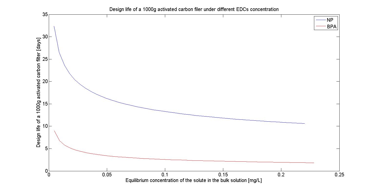
| − | The | + | The design life of filter under different EDCs concentration |
</p> | </p> | ||
<p> | <p> | ||
| − | To test The | + | To test The design life of filter under different maximum EDCs concentration, we first fixed our amount of activated carbon at 1000g and also fixed our maximum EDCs concentration at 10^(-6) M, 10^(-7) M, 10^(-8) M,and 10^(-9) M, which represent 2.2*10^(-1) mg/L, 2.2*10^(-2) mg/L, 2.2*10^(-3) mg/L, and 2.2*10^(-4) mg/L respectively. Based on the reference we found, we then assumed that the flow rate of water is 1.5L/sec and farmers will irrigate their farmland at the frequency of 7 days.Thus the total flow for each irrigation time will be 86400(sec)*7*1.5(L/sec)=907200(L).The results are shown in the following figures(Figure 24-27) : |
</p> | </p> | ||
<p> | <p> | ||
| − | <img width="90%"src="https://static.igem.org/mediawiki/2017/ | + | <img width="90%"src="https://static.igem.org/mediawiki/2017/0/08/T--NTHU_Taiwan--Model--Filter_design_life_12_EDC_concentration.png"> |
</p> | </p> | ||
| Line 601: | Line 620: | ||
<p> | <p> | ||
| − | <img width="90%"src="https://static.igem.org/mediawiki/2017/ | + | <img width="90%"src="https://static.igem.org/mediawiki/2017/9/9f/T--NTHU_Taiwan--Model--Filter_design_life_22_EDC_concentration.png"> |
</p> | </p> | ||
| Line 610: | Line 629: | ||
<p> | <p> | ||
| − | <img width="90%"src="https://static.igem.org/mediawiki/2017/ | + | <img width="90%"src="https://static.igem.org/mediawiki/2017/7/72/T--NTHU_Taiwan--Model--Filter_design_life_32_EDC_concentration.png"> |
</p> | </p> | ||
| Line 618: | Line 637: | ||
<p> | <p> | ||
| − | <img width="90%"src="https://static.igem.org/mediawiki/2017/ | + | <img width="90%"src="https://static.igem.org/mediawiki/2017/8/8d/T--NTHU_Taiwan--Model--Filter_design_life_42_EDC_concentration.png"> |
</p> | </p> | ||
| Line 624: | Line 643: | ||
<p><center><font size=2> | <p><center><font size=2> | ||
Figure 27. The design life vs EDCs concentration under the maxmium EDCs concentration of 2.2*10^(-4) mg/L | Figure 27. The design life vs EDCs concentration under the maxmium EDCs concentration of 2.2*10^(-4) mg/L | ||
| − | </font></center></p> | + | </font></center></p><br><br><br> |
<p> | <p> | ||
| − | We can see that as the concentration of EDCs increases, The | + | We can see that as the concentration of EDCs increases, The design life of filter decreases. It may because the more EDCs are presented in the water, the more activated carbon will bind to it, which then reduces the amount of activated carbon we can utilize and it proves that our filter can eliminate the EDCs in the lower concentration but it can’t afford the concentration of EDCs beyond the safe range. |
| − | </p> | + | </p><br><br><br> |
| Line 634: | Line 653: | ||
<center><h2> | <center><h2> | ||
Enzyme Kinetics | Enzyme Kinetics | ||
| − | </h2></center> | + | </h2></center><br> |
| + | |||
| + | <script src="https://gist.github.com/anonymous/4065f67ae3b79774a601b86faaff48ab.js"></script> | ||
| − | |||
| Line 644: | Line 664: | ||
<center><h2> | <center><h2> | ||
Freundlich Model | Freundlich Model | ||
| − | </h2></center> | + | </h2></center><br> |
| − | + | <script src="https://gist.github.com/anonymous/3668cd8c80b361855161a3621bdeb031.js"></script> | |
| − | + | <br> | |
| + | <br> | ||
| + | <br> | ||
| + | <h2>Reference</h2> | ||
| + | <br><br> | ||
| + | |||
| + | <p> | ||
| + | 1. Dong, S., Mao, L., Luo, S., Zhou, L., Feng, Y., & Gao, S. (2014). Comparison of lignin | ||
| + | peroxidase and horseradish peroxidase for catalyzing the removal of nonylphenol from the water. Environmental Science and Pollution Research, 21(3), 2358-2366. | ||
| + | </p> | ||
| + | <p> | ||
| + | 2. http://www.hccfa.org.tw/ | ||
| + | </p> | ||
| + | <p> | ||
| + | 3. Hamdaoui, O., & Naffrechoux, E. (2007). Modeling of adsorption isotherms of phenol and | ||
| + | chlorophenols onto granular activated carbon: Part I. Two-parameter models and equations | ||
| + | allowing determination of thermodynamic parameters. Journal of Hazardous materials, 147(1), | ||
| + | 381-394. | ||
| + | </p> | ||
| + | <p> | ||
| + | 4. Skopp, J. (2009). Derivation of the Freundlich adsorption isotherm from kinetics. J. Chem. | ||
| + | Educ, 86(11), 1341. | ||
| + | </p> | ||
| + | <p>5. Choi, K. J., Kim, S. G., Kim, C. W., & Kim, S. H. (2005). Effects of activated carbon types | ||
| + | and service life on the removal of endocrine disrupting chemicals: amitrole, nonylphenol, and | ||
| + | bisphenol-A. Chemosphere, 58(11), 1535-1545. | ||
| + | </p> | ||
Latest revision as of 16:24, 1 November 2017

Model
Overview1. Conducted Simulation in order to simulate filter’s working ability and improve our design. 2. Used the equation of Michaelis-Menten kinetics model to test our HRP degradation efficiency. 3. Derived Freundlich Adsorption Isotherm model to measure the adsorption capacity of our filter. 4. Modeled the design life of our filter to predict the frequency of replacement of inner activated carbons. |
Model 1: Enzyme kinetics
Theory and derivation of enzyme kinetics :
We simplified our enzyme-EDCs system as the reaction with the process of the first and second order reactions:

The initial collision of E (Enzyme) and S (Substrate) is a bimolecular reaction with the second-order rate constant k1. The ES complex can then undergo one of two possible reactions: k2 is the first-order rate constant for the conversion of ES to E and P, and k-1 is the first-order rate constant for the conversion of ES back to E and S.We assume that the formation of product from ES (the step described by k2) does not occur in reverse.
The rate equation for product formation is:

However, measuring [ES] is more difficult because the concentration of the enzyme-substrate complex depends on its rate of formation from E and S and its rate of decomposition to E + S and E + P:

To simplify our analysis, we choose experimental conditions such that the substrate concentration is much greater than the enzyme concentration and ES remains constant until nearly all the substrate has been converted to product.

According to the steady-state assumption, the rate of ES formation must therefore balance the rate of ES consumption:

The total enzyme concentration, [E]T, is usually known:

This expression for [E] can be substituted into the rate equation to give:

Rearranging (by dividing both sides by [ES] and k1) gives an expression in which all three rate constants are together:

We defined KM and rearranged the equation:

We did some compute process for the equation and give:

Solving for [ES],

Finally, we can express the reaction velocity as:

The maximum reaction velocity, Vmax, can be expressed as:

And then we can get the equation,

In order to estimate the degradation capacity of the filter, we calculated horseradish peroxidase’s ability of degradation based on the equation of Michaelis-Menten kinetics :
The degradation rate under different EDCs concentration
We used several parameters according to the paper we found to calculate the initial velocity of different concentrations of BPA and NP. Also, their concentrations at different time after starting degradation.
NP:
[H2O2]=10^(-5) M
Km=10.1*10^(-6) M
Vmax=0.056*10^(-6) M/s
S=9.1*10^(-10)~9.1*10^(-6) M
BPA:
[H2O2]=0.02*10^(-3) M
Km=6*10^(-6) M
Vmax=2.22*10^(-9) M/s
S=8.77*10^(-10)~8.77*10^(-6) M
The results are shown in the following figures(Figure 1-4) :


From the results of the enzyme kinetics, we can find that when the concentration of EDCs increases, the degradation rate increases dramatically. As a result, our activated carbon in the system of our filter can help HRP to degrade EDCs in the more efficient way since its outstanding ability to capture EDCs in the water and accumulate more EDCs around HRP.
To prove the accumulative ability of activated carbon
To prove that our activated carbon can effectively accumulate our EDCs, we compared the time duration for 50%,75%, and 95% degradation between different concentrations of EDCs in the unsaturated activated carbon and those in the saturated activated carbon. (Since we believed that if our activated carbon can effectively accumulate EDCs, the EDCs solution should we saturated)
We fixed the EDCs solution at the concentrations of 10^(-6) M,10^(-7) M,10^(-8) M, and 10^(-9) M. (not in the activated carbon)The results are shown in the following figures(Figure 5-19) :


As we can see in the results, the scale of time duration for degrading the unsaturated EDCs solution can up to 10^(15) sec, however, the time duration for degrading the saturated EDCs solution are only 10^(10)sec. This proves that our filter can effectively accumulate EDCs to let our enzyme degrade much more faster.
Model 2: Concentration Test
Theory and derivation of the Freundlich Adsorption Isotherm from Kinetics
In general, the rate law can be written as:

If we imagine a small pore, adsorption sites near the open ends are different from at the center of the pore. This distinction occurs when the sites possess specific chemical properties. If a concentration is imposed at one end of the pore, solute must diffuse to find an open adsorption site first and it is similar as the desorption case.In this point, the exponent n is a measure of the fractal dimension of the process and the rate constant for fractal reactions is also expected to be proportional to the molecular diffusion coefficient.For both adsorption and desorption reactions but with distinct fractal dimensions (ni) and fractal rate constants (ki):

At equilibrium, the derivative is equal to zero and the equation can then be solved for S:

Finally, we can transform the equation to the Freundlich Adsorption equation,

Ce : the equilibrium concentration of the solute in the bulk solution (mg L−1)(the concentration of EDCs)
KF : Freundlich constant indicative of the relative adsorption capacity of the adsorbent (mg1−(1/n) L1/n g−1)
n : Freundlich constant indicative of the intensity of the adsorption
qe: the amount of solute adsorbed per unit weight of adsorbent at equilibrium (mg g−1)(the maximum of the adsorption)
To further estimate our filter’s function, we’ve conducted two models based on the Freundlich Adsorption equation as following:
The adsorption capacity under different EDCs concentration
To test the adsorption capacity under different maximum EDCs concentration, we than fixed our maximum EDCs concentration as Ce at 10^(-6) M, 10^(-7) M, 10^(-8) M,and 10^(-9) M, which represent 2.2*10^(-1) mg/L, 2.2*10^(-2) mg/L, 2.2*10^(-3) mg/L, and 2.2*10^(-4) mg/L respectively. The results are shown in the following figures(Figure 20-23) :


We can see that as the concentration of EDCs (Ce) increases, the adsorption amount per unit weight of adsorbent at eq. also increases. We deduced that it might because as the concentration arises, the collision frequency between EDCs and our activated carbon increases, leading to the higher amount of adsorbent.
The design life of filter under different EDCs concentration
To test The design life of filter under different maximum EDCs concentration, we first fixed our amount of activated carbon at 1000g and also fixed our maximum EDCs concentration at 10^(-6) M, 10^(-7) M, 10^(-8) M,and 10^(-9) M, which represent 2.2*10^(-1) mg/L, 2.2*10^(-2) mg/L, 2.2*10^(-3) mg/L, and 2.2*10^(-4) mg/L respectively. Based on the reference we found, we then assumed that the flow rate of water is 1.5L/sec and farmers will irrigate their farmland at the frequency of 7 days.Thus the total flow for each irrigation time will be 86400(sec)*7*1.5(L/sec)=907200(L).The results are shown in the following figures(Figure 24-27) :


We can see that as the concentration of EDCs increases, The design life of filter decreases. It may because the more EDCs are presented in the water, the more activated carbon will bind to it, which then reduces the amount of activated carbon we can utilize and it proves that our filter can eliminate the EDCs in the lower concentration but it can’t afford the concentration of EDCs beyond the safe range.
Enzyme Kinetics
Freundlich Model
Reference
1. Dong, S., Mao, L., Luo, S., Zhou, L., Feng, Y., & Gao, S. (2014). Comparison of lignin peroxidase and horseradish peroxidase for catalyzing the removal of nonylphenol from the water. Environmental Science and Pollution Research, 21(3), 2358-2366.
2. http://www.hccfa.org.tw/
3. Hamdaoui, O., & Naffrechoux, E. (2007). Modeling of adsorption isotherms of phenol and chlorophenols onto granular activated carbon: Part I. Two-parameter models and equations allowing determination of thermodynamic parameters. Journal of Hazardous materials, 147(1), 381-394.
4. Skopp, J. (2009). Derivation of the Freundlich adsorption isotherm from kinetics. J. Chem. Educ, 86(11), 1341.
5. Choi, K. J., Kim, S. G., Kim, C. W., & Kim, S. H. (2005). Effects of activated carbon types and service life on the removal of endocrine disrupting chemicals: amitrole, nonylphenol, and bisphenol-A. Chemosphere, 58(11), 1535-1545.