| Line 171: | Line 171: | ||
<p>This model was designed to calculate the maximum efficiency of a Split YFP system, assuming the aggregates are very long.</p> | <p>This model was designed to calculate the maximum efficiency of a Split YFP system, assuming the aggregates are very long.</p> | ||
<object width="100%" height="800px" data="https://static.igem.org/mediawiki/2017/c/c2/Sup35_Split_YFP_Amyloids_as_a_Markov_Chain.pdf"></object> | <object width="100%" height="800px" data="https://static.igem.org/mediawiki/2017/c/c2/Sup35_Split_YFP_Amyloids_as_a_Markov_Chain.pdf"></object> | ||
| + | </div></div></div> | ||
| + | </div> | ||
| + | <div class="row subProject" v-if="ip.showing=='FRET Conversion'"> | ||
| + | <div class="row"><div class="col"><div class="content-main"><h1 id="fret-efficiency-conversion">FRET Efficiency Conversion</h1> | ||
| + | <p>One of the most significant potential applications of our project is in substrate channelling. This model aims to use FRET measurements as a method for predicting the efficiency of a potential substrate channelling system.</p> | ||
| + | <object width="100%" height="800px" data="https://static.igem.org/mediawiki/2017/0/03/FRET_efficiency_conversion.pdf"></object> | ||
</div></div></div> | </div></div></div> | ||
</div> | </div> | ||
| Line 200: | Line 206: | ||
{ title: "Combinatorial Model" }, | { title: "Combinatorial Model" }, | ||
{ title: "Markov Model" }, | { title: "Markov Model" }, | ||
| + | { title: "FRET Conversion" }, | ||
] | ] | ||
}}} | }}} | ||
Latest revision as of 01:10, 2 November 2017
Model
An important property to understand in the implementation of our project is the upper bound for the efficiency of a given system.
There are two parts to this problem. First, we look at how aggregates are likely to form in time. Second, we examine how the ordering of proteins within an aggregate affects the overall efficiency of the system, and determine the expected value of this efficiency assuming the proteins join the aggregate at random.
Calculating these values allowed us to prioritize which experiments to devote lab resources to and gave us a better understanding of the systems we were studying. Additionally, similar techniques may be applied to judge the efficiency of new applications of our project.
Protein aggregation molecular differential equation model
Full Network Model
The goal was to create a model that could predict the size of the aggregated protein. To create the model we used a method outlined in the text Mathematical Modelling in Systems Biology: An Introduction. [^1] A graphic representation of our model is shown below.
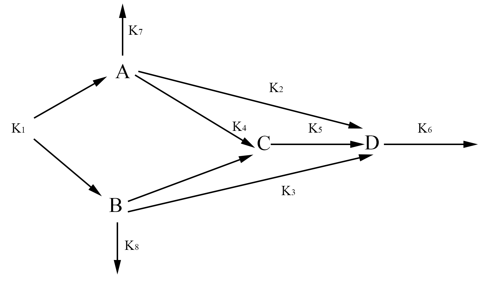
In our model, we have labeled one half of FYP as A and the other half as B. A and B may come together to form a dimer C. The dimer and singular half pieces A and B all aggregate into the final protein product D. The rate the cell creates A and B is represented by the rate constant k1. The degradation of A and B is represented by the rate constants k7 and k8 respectively. The formation of the dimer is represented by the rate constant k4. The rate at which C, A, and B join into the final protein product D is represented by the rate constants k5, k2, and k3 respectively. Finally, the rate at which the protein aggregates degrades is represented by the rate constant k6. With the rate constants, we may use chemical mass actions kinetics to represent our model with a system of differential equations as follows.
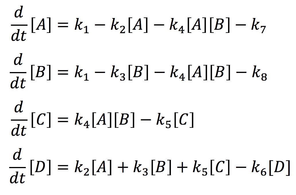
If we solve this system numerically and graph it we get the fallowing graph.
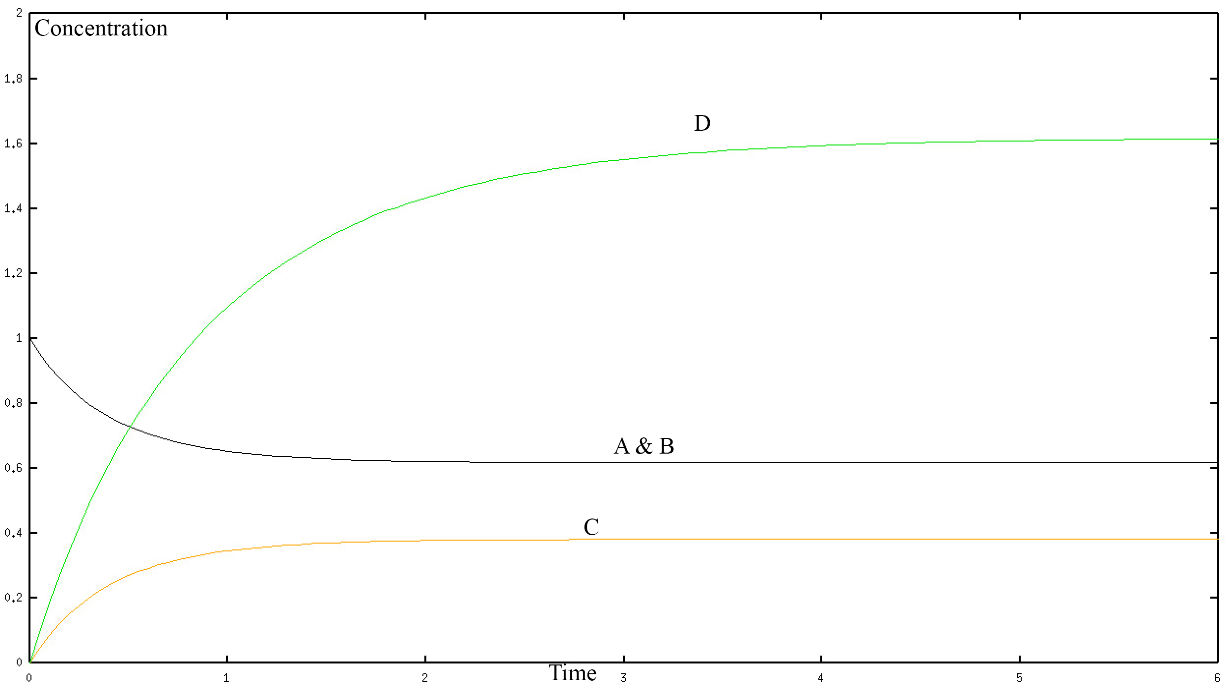
In the graph, the black curve represents the concentration of A and B with respect to time. The yellow curve represents the concentration of C with respect to time. The green curve represents the connection of D with respect to time. The concentration is in mol/L and time is in seconds. D is one protein so a “higher concentration of D” simply represents a larger protein. The numerical values shown in the graph are not important here and may not be accurate, they depend on the rate constants k1-k8 of our system, which is unknown. Rather the graph allows us to see the long-term behaviour of the different proteins in our model. Clearly, we can see that they all reach a steady state. That is to say that at a certain point the protein's contention does not change with time. Therefore, our model is making a prediction that makes sense when compared to reality, which gives us confidence that we are on the right track. However, the model as we have stated it thus far can only be solved numerically not analytically. Therefore let us create a simplified version of the model.
Simplified network model
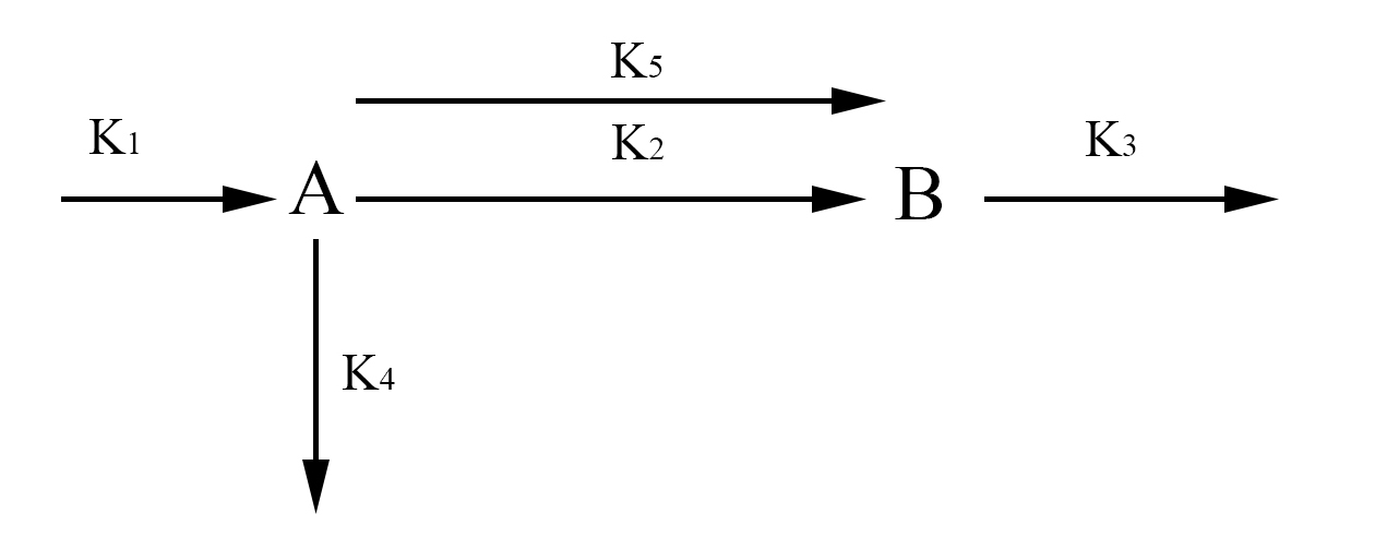
In the simplified model rather than representing each half of FYP as A and B, we will represent it simply as one protein A. This simplification is valid because the dynamics of A and B are exactly the same. The aggregate protein is represented by B. The rate at which A is formed and degraded is represented by the rate constants k1 and k4 respectively. We will represent A turning into a dimer and joining the aggregate B with the rate constant k2. A can also join the aggregate as a single protein rather than a dimer which will be represented with the rate constant k5. Finally, we will represent the degradation of B with the rate constant k3. Again we use chemical mass actions kinetics to represent the simplified model with a system of differential equations, as fallows.

This system can be solved analytically if one assumes that at some point the concentration of A will no longer change. This assumption is valid from the graph earlier where we observed that all the protein systems reached steady state. Hence with the steady-state assumption, we can solve the system analytically as fallows.
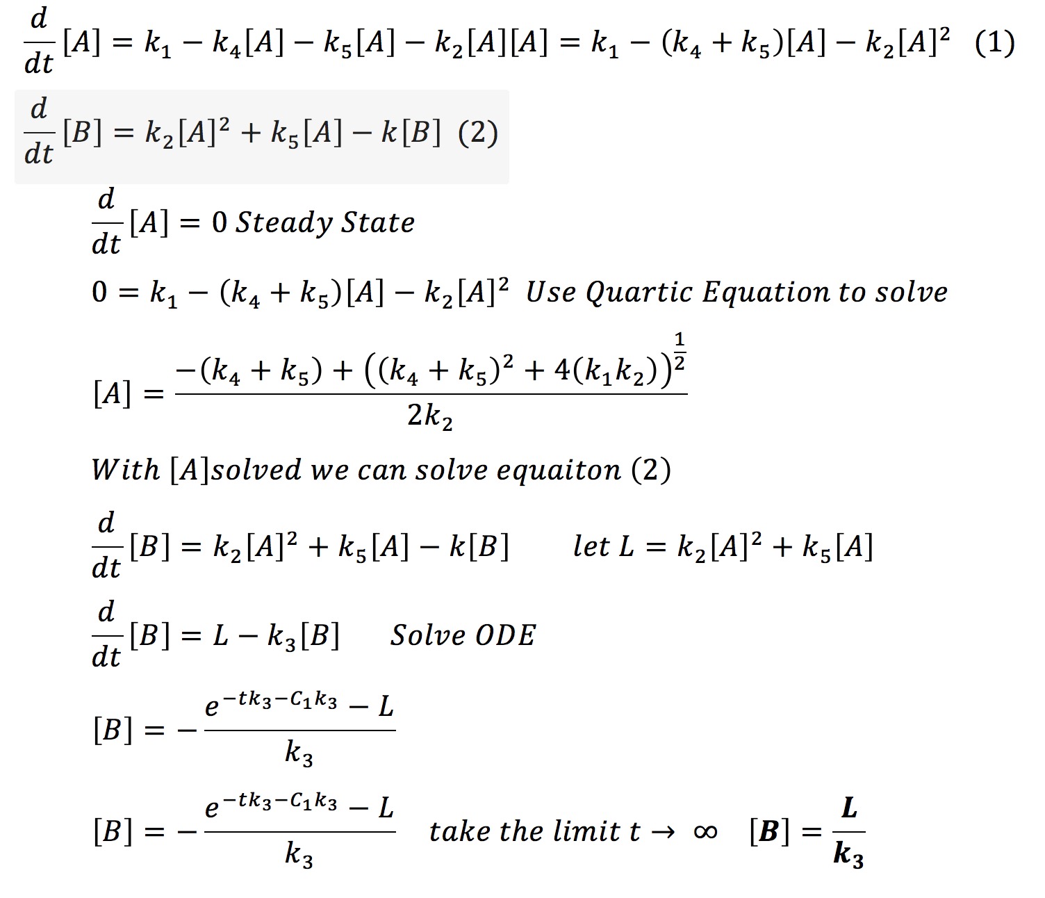
Therefore it is possible that if one knows the final amount of aggregated protein [B] and if one knows the rate of degradation of that protein k3 one can find a constant L. With that constant and k3 it is possible to always know the amount of aggregate we will have in our system.
[^1]: Ingalls, B. P. (2013). Mathematical modeling in systems biology: An introduction. Cambridge, MA: The MIT Press.
Combinatorial Model
This model was designed to calculate the maximum efficiency of a Split YFP or FRET system, for aggregates of length n.
Markov Model
This model was designed to calculate the maximum efficiency of a Split YFP system, assuming the aggregates are very long.
FRET Efficiency Conversion
One of the most significant potential applications of our project is in substrate channelling. This model aims to use FRET measurements as a method for predicting the efficiency of a potential substrate channelling system.

