Difference between revisions of "Team:UiOslo Norway/Modelling"
| (44 intermediate revisions by 4 users not shown) | |||
| Line 9: | Line 9: | ||
</head> | </head> | ||
| − | <h1 class="h1-font-other"> | + | <h1 class="h1-font-other">Modelling</h1> |
<div class="bootstrap-overrides padding-left padding-right"> | <div class="bootstrap-overrides padding-left padding-right"> | ||
| + | |||
| + | |||
| Line 17: | Line 19: | ||
<div class="col-md-12"> | <div class="col-md-12"> | ||
<ul id="tab2" class="nav nav-pills"> | <ul id="tab2" class="nav nav-pills"> | ||
| − | <li class="active"><a href="#tab-item1" data-toggle="tab"> | + | <li class="active"><a href="#tab-item1" data-toggle="tab">Light</a></li> |
| − | <li><a href="#tab-item2" data-toggle="tab"> | + | <li><a href="#tab-item2" data-toggle="tab">LED</a></li> |
| − | <li><a href="#tab-item3" data-toggle="tab"> | + | <li><a href="#tab-item3" data-toggle="tab">Setup</a></li> |
| − | <li><a href="#tab-item4" data-toggle="tab"> | + | <li><a href="#tab-item4" data-toggle="tab">Lasing</a></li> |
| − | + | ||
| − | + | ||
| − | + | ||
| − | + | ||
| − | + | ||
| − | + | ||
| − | + | ||
</ul> | </ul> | ||
| Line 35: | Line 30: | ||
<div class="tab-pane fade active in" id="tab-item1"> | <div class="tab-pane fade active in" id="tab-item1"> | ||
<br> <br> | <br> <br> | ||
| − | <div class="bootstrap-overrides | + | <div class="bootstrap-overrides-with-pictures"> |
| − | + | <div class="modelling-content"> | |
| − | + | ||
| − | + | ||
| − | + | ||
| − | + | ||
| − | + | ||
| − | + | ||
| − | + | ||
| − | + | ||
| − | + | ||
| − | + | ||
| − | + | ||
| − | + | ||
| − | + | ||
| − | + | ||
| − | + | ||
| − | + | ||
| − | + | ||
| − | + | ||
| − | + | ||
| − | + | ||
| + | <div class="padding-right padding-left"> | ||
| + | Electromagnetic radiation is energy travelling as waves or photons. This is not the time or the place to go into this discussion [1] but Einstein and Infeld said it well: <br><br> | ||
| + | </div> | ||
| + | <div class="padding-right padding-left"> | ||
| + | <div class="media-body"> | ||
| + | <blockquote> | ||
| + | "But what is light really? Is it a wave or a shower of photons? There seems no likelihood for forming a consistent description of the phenomena of light by a choice of only one of the two languages. It seems as though we must use sometimes the one theory and sometimes the other, while at times we may use either. We are faced with a new kind of difficulty. We have two contradictory pictures of reality; separately neither of them fully explains the phenomena of light, but together they do." </blockquote> | ||
| + | <h3><a href="#" class="bodyURLcolor">- Albert Einstein and Leopold Infeld, The Evolution of Physics, pg. 262-263.</a></h3> | ||
| + | </div> | ||
| + | </div><br> <br> | ||
| + | <div class="padding-right padding-left"> | ||
| + | Light, or the visible light spectrum range from \( \in [400 - 700] \) nm in the electromagnetic radiation spectrum. | ||
| + | Above, with higher wavelengths, you will find infrared radiation (also known as IR), and under you will find the ultraviolet radiation (also known as UV). We call it <i>visible light</i> due to the fact that our eyes can only "pick up" these wavelengths. For this project we will mostly focus on light \( \lambda \in [470,520] \) nm region. | ||
| + | </div> | ||
| + | <div class="padding-right padding-left"> | ||
| + | <br> | ||
| + | You have probably heard that nothing can travel faster than light? But not that many (non-physicist) remembers what velocity light actually travels with. In most cases it's enough to say that light travels in \( \sim 3.0 \cdot 10^{8}\) m/s in vacuum or \( \sim 6.7 {\cdot 10^{8}} \)mph. | ||
| + | </div> | ||
| + | |||
| + | <!-- Insert picture of spectrometer set up--> | ||
| + | <div class="padding-right padding-left"> | ||
| + | <br> | ||
| + | The given wavelength \(\lambda \) for a lightsource can be found using the following formula: | ||
| + | </div> | ||
| + | <div class= "padding-right padding-left"> | ||
| + | \begin{align} | ||
| + | \lambda = d sin(\theta) | ||
| + | \end{align} | ||
| + | </div> | ||
| + | <div class="padding-right padding-left"> | ||
| + | Where \(d\) is the grid spacing and \(\theta\) is the angle. | ||
| + | </div> | ||
| + | <div class="padding-right padding-left" > | ||
| + | <br> | ||
| + | Continuing this part we will refer to light as waves. As shown in the picture above, visible light ranges around ∈[400−700] nm. This is known as the wavelength of the light, and to label it we use the symbol \(\lambda\). To better understand the physics we will start by using the rainbow as an example. Most people have had the pleasure to see this magnificent phenomenon in their life. To understand what happens to the light, we need to introduce the term refraction index. In short terms, this means that light will behave differently in different mediums if hit with an angle different than zero from the optical path. For air, the refraction index is simply \(1\), but for water it is \(1.33\), both in vacuum. Using Snell’s law and the fact that the light travels from air to water we can see that the angle with which the light will be emitted can be found by: | ||
| + | </div> | ||
| + | <div class="padding-right padding-left"> | ||
| + | \begin{align} | ||
| + | n_1 sin\theta_1 = n_2 sin\theta_2 | ||
| + | \end{align} | ||
| + | </div> | ||
| + | <div class="padding-left padding-top"> | ||
| + | <h1 class="padding-right padding-left">References</h1> | ||
| + | [1] <a href="https://en.wikipedia.org/wiki/Wave%E2%80%93particle_duality" class="bodyURLcolor"> if you want to read more about the waves vs. photons disussion </a><br> | ||
| + | [2] Vistnes, A. (2016). Svingninger og Bølgers Fysikk. CreateSpace, An Amazone.com Company | ||
| + | </div> | ||
| + | </div> | ||
| + | <div class="modelling-picture"> | ||
| + | <figure> | ||
| + | <img class="team-picture" src = "https://static.igem.org/mediawiki/2017/f/f8/T--UiOslo_norway--modelling_spectrum.png"> | ||
| + | <figcaption>The electromagnetic spectrum for the electromagnetic radiation with the corresponding wavelengths.</figcaption> | ||
| + | </figure> | ||
| − | + | </div> | |
| − | + | ||
| − | + | ||
| − | + | ||
| − | + | ||
| − | + | ||
| − | + | ||
| − | + | ||
| − | + | ||
| − | + | ||
| − | + | ||
| − | + | ||
| − | + | ||
| − | + | ||
| − | + | ||
| − | + | ||
| − | + | ||
| − | + | ||
</div> | </div> | ||
</div> | </div> | ||
| Line 83: | Line 94: | ||
| − | |||
| − | |||
| − | + | <div class="tab-pane fade" id="tab-item2"> | |
| − | + | ||
| − | + | ||
| − | + | ||
| − | + | ||
| − | + | ||
| − | + | ||
| − | + | ||
| − | + | ||
| − | + | ||
| − | + | ||
| − | + | ||
| − | + | ||
| − | + | ||
| − | + | ||
| − | + | ||
| − | + | ||
| − | + | ||
| − | + | ||
| − | + | ||
| − | + | ||
| − | + | ||
| − | + | ||
| − | + | ||
| − | + | ||
| − | + | ||
| − | + | ||
| − | + | ||
| − | + | ||
| − | + | ||
| − | + | ||
| − | + | ||
| − | + | ||
| − | + | ||
| − | + | ||
| − | + | ||
| − | + | ||
| − | + | ||
| − | + | ||
| − | + | ||
| − | + | ||
| − | + | ||
| − | + | ||
| − | + | ||
| − | + | ||
| − | + | ||
| − | + | ||
| − | + | ||
| − | + | ||
| − | + | ||
| − | + | ||
| − | + | ||
| − | + | ||
| − | + | ||
| − | + | ||
| − | + | ||
| − | + | ||
| − | + | ||
| − | + | ||
| − | + | ||
| − | + | ||
| − | + | ||
| − | + | ||
| − | + | ||
| − | + | ||
| − | + | ||
| − | + | ||
| − | + | ||
| − | + | ||
| − | + | ||
| − | + | ||
| − | + | ||
| − | + | ||
| − | + | ||
| − | + | ||
| − | + | ||
| − | + | ||
| − | + | ||
| − | + | ||
| − | + | ||
| − | + | ||
| − | + | ||
| − | + | ||
| − | + | ||
| − | + | ||
| − | + | ||
| − | + | ||
| − | + | ||
| − | + | ||
| − | + | ||
| − | + | ||
| − | + | ||
| − | + | ||
| − | + | ||
| − | + | ||
| − | + | ||
| − | + | ||
| − | + | ||
| − | + | ||
| − | + | ||
| − | + | ||
| − | + | ||
| − | + | ||
| − | + | ||
| − | + | ||
| − | + | ||
| − | + | ||
| − | + | ||
| − | + | ||
| − | + | ||
| − | + | ||
| − | + | ||
| − | + | ||
| − | + | ||
| − | + | ||
| − | + | ||
| − | + | ||
| − | + | ||
| − | + | ||
| − | + | ||
| − | + | ||
| − | + | ||
| − | + | ||
| − | + | ||
| − | + | ||
| − | + | ||
| − | + | ||
| − | + | ||
| − | + | ||
| − | + | ||
| − | + | ||
| − | + | ||
| − | + | ||
| − | + | ||
| − | + | ||
| − | + | ||
| − | + | ||
| − | + | ||
| − | + | ||
| − | + | ||
| − | + | ||
| − | + | ||
| − | + | ||
| − | + | ||
| − | + | ||
| − | + | ||
| − | + | ||
| − | + | ||
| − | + | ||
| − | + | ||
| − | + | ||
| − | + | ||
| − | + | ||
| − | + | ||
| − | + | ||
| − | + | ||
| − | + | ||
| − | + | ||
| − | + | ||
| − | + | ||
| − | + | ||
| − | + | ||
| − | + | ||
| − | + | ||
| − | + | ||
| − | + | ||
| − | + | ||
| − | + | ||
| − | + | ||
| − | + | ||
| − | + | ||
| − | + | ||
| − | + | ||
| − | + | ||
| − | + | ||
| − | + | ||
| − | + | ||
| − | + | ||
| − | + | ||
| − | + | ||
| − | + | ||
| − | + | ||
| − | + | ||
| − | + | ||
| − | + | ||
| − | + | ||
| − | + | ||
| − | + | ||
| − | + | ||
| − | + | ||
| − | + | ||
| − | + | ||
| − | + | ||
| − | + | ||
| − | + | ||
| − | + | ||
| − | + | ||
| − | + | ||
| − | + | ||
| − | + | ||
| − | + | ||
| − | + | ||
| − | + | ||
| − | + | ||
| − | + | ||
| − | + | ||
| − | + | ||
| − | + | ||
| − | + | ||
| − | + | ||
| − | + | ||
| − | + | ||
| − | + | ||
| − | + | ||
| − | + | ||
| − | + | ||
| − | + | ||
| − | + | ||
| − | + | ||
| − | + | ||
| − | + | ||
| − | + | ||
| − | + | ||
| − | + | ||
| − | + | ||
| − | + | ||
| − | + | ||
| − | + | ||
| − | + | ||
| − | + | ||
| − | + | ||
| − | + | ||
| − | + | ||
| − | + | ||
| − | + | ||
| − | + | ||
| − | + | ||
| − | + | ||
| − | + | ||
| − | + | ||
| − | + | ||
| − | + | ||
| − | + | ||
| − | + | ||
| − | + | ||
| − | + | ||
| − | + | ||
| − | + | ||
| − | + | ||
| − | + | ||
| − | + | ||
| − | + | ||
| − | + | ||
| − | + | ||
| − | + | ||
| − | + | ||
| − | + | ||
| − | + | ||
| − | + | ||
| − | + | ||
| − | + | ||
| − | + | ||
| − | + | ||
| − | + | ||
| − | + | ||
| − | + | ||
| − | + | ||
| − | + | ||
| − | + | ||
| − | + | ||
| − | + | ||
| − | + | ||
| − | + | ||
| − | <div class="tab-pane fade | + | |
<br> <br> | <br> <br> | ||
| Line 365: | Line 101: | ||
<div class="modelling-content"> | <div class="modelling-content"> | ||
| − | |||
| − | |||
| − | |||
| − | |||
| − | |||
| − | |||
| − | |||
| − | |||
| − | |||
| − | |||
| − | |||
| − | |||
| − | |||
| − | |||
| − | |||
| − | |||
| − | |||
| − | |||
| − | |||
| − | |||
| − | |||
| − | |||
| − | |||
| − | |||
| − | |||
| − | |||
| − | |||
| − | |||
| − | |||
| − | |||
| − | |||
| − | |||
| − | |||
| − | |||
| − | |||
| − | |||
| − | |||
| − | |||
| − | |||
| − | |||
| − | |||
| − | |||
| − | |||
| − | |||
| − | |||
| − | |||
| − | |||
| − | |||
| − | |||
| − | |||
| − | |||
| − | |||
| − | |||
| − | |||
| − | |||
| − | |||
| − | |||
| − | |||
| − | |||
| − | |||
| − | |||
| − | |||
| − | |||
| − | |||
| − | |||
| − | |||
| − | |||
| − | |||
| − | |||
| − | |||
| − | |||
| − | |||
| − | |||
| − | |||
| − | |||
| − | |||
| − | |||
| − | |||
| − | |||
| − | |||
| − | |||
| − | |||
| − | |||
| − | |||
| − | |||
| − | |||
| − | |||
| − | |||
| − | |||
| − | |||
| − | |||
| − | |||
| − | |||
| − | |||
| − | |||
| − | |||
| − | |||
| − | |||
| − | |||
| − | |||
| − | |||
| − | |||
| − | |||
| − | |||
| − | |||
| − | |||
| − | |||
| − | |||
| − | |||
| − | |||
| − | |||
| − | |||
| − | |||
| − | |||
| − | |||
| − | |||
| − | |||
| − | |||
| − | |||
| − | |||
| − | |||
| − | |||
| − | |||
| − | |||
| − | |||
| − | |||
| − | |||
| − | |||
| − | |||
| − | |||
| − | |||
| − | |||
| − | + | <div class="padding-right padding-left"> | |
| − | + | The light from a light-emitting diode, LED for short, can be viewed by the human eye as monochromatic. This means it appears to only light up as one color. From theory we know that a LED cannot be monochromatic, thus proving one of the biggest differences between a LED and a laser. More importantly, the light from a LED is not coherent, meaning that the light waves do not have the same frequency. A LED loses little energy to heat as it applies most of its energy to light up the diode. This is a very useful property.<br><br> | |
| − | + | </div> | |
| − | + | <div class="padding-right padding-left"> | |
| − | + | To create a simple LED-circuit you only need a couple of components: a LED, a resistance, some wires, a circuit board and a voltage source. | |
| − | + | </div> | |
| − | </ | + | |
</div> | </div> | ||
| − | + | <div class="modelling-picture"> | |
<figure> | <figure> | ||
| − | + | <img class="modelling-picture" src = "https://static.igem.org/mediawiki/2017/5/52/T--UiOslo_norway--modelling_LEDcircuit.png"> | |
| − | + | <figcaption> Illustration of our LED circuit. With a resistance, a LED and two power wires for both the positive and negative current. </figcaption> | |
</figure> | </figure> | ||
</div> | </div> | ||
| Line 517: | Line 120: | ||
</div> | </div> | ||
| − | |||
| − | |||
| − | |||
| − | |||
| − | |||
| − | |||
| − | |||
| − | |||
| − | |||
| − | |||
| − | |||
| − | |||
| − | |||
| − | |||
| − | |||
| − | |||
| − | |||
| − | |||
| − | <div class="tab-pane fade | + | <div class="tab-pane fade" id="tab-item3"> |
| − | + | ||
| − | + | ||
| − | + | ||
| − | + | ||
| − | + | ||
| − | + | ||
| − | + | ||
| − | + | ||
| − | + | ||
| − | + | ||
| − | + | ||
| − | + | ||
| − | + | ||
<br> <br> | <br> <br> | ||
| Line 556: | Line 128: | ||
<div class="modelling-content"> | <div class="modelling-content"> | ||
| − | + | ||
| − | + | As one can see in the figure, our setup contains the following components: a LED-circuit as light source, lenses, two color filters, two mirrors, a spectrometer and a CCD-camera. The purpose of the lenses is to focus the light from the LED-circuit into a thin beam. This will make the LED-light more similar to a laser, and also increase the intensity of the light by concentrating it into a smaller radius. In order to make our light source act more like a laser, we need the light to have monochromatic properties. By using a blue color filter we can remove some of its spectrum, and obtain a correct wavelength for the GFP and yeast. It is worth mentioning that even though we use filters and lenses to focus the light, we still have to keep the LED at a maximum of 20V and hopefully the intensity is high enough for lasing to happen. Ideally, the mirrors we use should be 98% reflective and the last 2% should be emitted light that we can detect. We were not able to acquire mirrors of that sort, which is why our setup looks a bit different from that of a regular laser. The solution (both GFP or yeast) will be placed between the mirrors, in order to increase the effect of the light emitted from the solution. To be able to gather the light emitted from the GFP, which will be emitted in all directions, we place a big lense next to the mirror chamber. This lense will focus the light from the solution into a filter that removes the wavelengths that belongs to the LED, and by that we obtain the wavelengths we want to observe in a spectrometer or CCD-camera. | |
| − | + | ||
| − | + | ||
| − | + | ||
| − | + | ||
| − | + | ||
| − | + | ||
| − | + | ||
</div> | </div> | ||
| − | |||
<div class="modelling-picture"> | <div class="modelling-picture"> | ||
<figure> | <figure> | ||
| − | + | <img class="modelling-picture" src = "https://static.igem.org/mediawiki/2017/9/99/T--UiOslo_norway--modelling_set_up.png"> | |
| − | + | <figcaption> Illustration of our set up. From left to right we start with the LED-circuit, which emmits light that travels through a blue filter, then a couple of lenses to parallel and gather the light before it hits the sample. Here we have our two mirrors to amplify the signal from the sample, and further down the optical path we use a big lens to gather as much light as possible to concentrate it to our green filter before we use our spectrometer (and if needed a CCD-camera) to gather information about the light.</figcaption> | |
| − | + | ||
| − | + | ||
| − | + | ||
| − | + | ||
</figure> | </figure> | ||
</div> | </div> | ||
| Line 581: | Line 141: | ||
</div> | </div> | ||
| − | <div class="tab-pane fade | + | |
| + | <div class="tab-pane fade" id="tab-item4"> | ||
<br> <br> | <br> <br> | ||
| − | <div class="bootstrap-overrides | + | <div class="bootstrap-overrides"> |
| − | + | ||
| − | + | ||
| − | + | ||
| + | <div class="padding-right padding-left"> | ||
| + | To be able to separate the fluoresence and the lasing with our setup we need to look at the spectre of the light waves emitted from the solution we are working with. The spectre of GFP is a broad peak as opposed to the laser, which has only one clear peak. When looking at our spectre we need to look for the clear peak, the laser peak. This will prove that we have succeeded in making the proteins lase, which will hopefully result in us proving the concept of a biolaser. <br> | ||
| + | <br> | ||
| + | Our CCD-camera do not have a lense, only a detector in place. In order to know if we will get an image we can see and work with, we need to calculate how big the detected image potentially will be. We are working with wavelengths that go roughly from 505 nm-515 nm, so we wish to calculate the angle between the two waves when they pass through the slit of the spectrometre. We also know that 4000 bars occupy a space of 2.5 cm, so we can calculate \(d\): | ||
</div> | </div> | ||
| + | <div class="padding-right padding-left"> | ||
| + | \begin{align} | ||
| + | d = 2.5 \cdot 10^{-3} / 4000 = 6.25 \cdot 10^{-6} m \\ | ||
| + | \theta = sin^{-1} \left(\frac{505 \cdot 10^{-9}m}{6.25 \cdot 10^{-6}m}\right) = 0.081 rad \\ | ||
| + | \phi = sin^{-1} \left(\frac{515 \cdot 10^{-9} m}{6.25 \cdot 10^{-3}}\right) = 0.082 rad | ||
| + | \end{align} | ||
| + | </div> | ||
| + | <div class="padding-right padding-left"> | ||
| + | The distance from the grid to the tip of the spectrometre (where we would out our camera) is 0.3m. So, the space between the two waves (and so, the size of our image) is: | ||
| + | </div> | ||
| + | <div class="padding-right padding-left"> | ||
| + | \begin{align} | ||
| + | (0.082 - 0.081) \cdot 0.3m = 0.3mm | ||
| + | \end{align} | ||
| + | </div> | ||
| + | <div class="padding-right padding-left"> | ||
| + | It is also worth mentioning that the angle at which the waves pass through the grid is more or less 5 degrees. To check if this works with our camera, we take the number of pixels pr 5 mm, and get: | ||
| + | </div> | ||
| + | <div class="padding-right padding-left"> | ||
| + | \begin{align} | ||
| + | \frac{0.005 m}{750 px} = 6.67 \cdot 10^{-6} = 7 \mu m | ||
| + | \end{align} | ||
| + | </div> | ||
| + | <div class="padding-right padding-left"> | ||
| + | Anything bigger than 7 \(\mu \) m should be easily observed, and our image should project at around 0.3 mm, so we are good to go! This is where the spectrometre and the CCD camera come into play. By knowing more or less the angle at which the spectre will be emitted we can place the camera where the spectre is sure to appear, and get a good measure of the spectre on screen. | ||
| − | |||
| − | |||
| − | |||
| − | |||
| − | |||
| − | |||
| − | |||
| − | |||
| − | |||
| − | |||
| − | |||
| − | |||
| − | |||
| − | |||
| − | |||
| − | |||
| − | |||
| − | |||
| − | |||
| − | |||
| − | |||
| − | |||
| − | |||
| − | |||
| − | |||
| − | |||
| − | |||
| − | |||
| − | |||
| − | |||
| − | |||
| − | |||
| − | |||
| − | |||
| − | |||
| − | |||
| − | |||
| − | |||
| − | |||
| − | |||
| − | |||
| − | |||
| − | |||
| − | |||
| − | |||
| − | |||
| − | |||
| − | |||
</div> | </div> | ||
</div> | </div> | ||
</div> | </div> | ||
| − | |||
| − | |||
| − | |||
</div> | </div> | ||
Latest revision as of 03:49, 2 November 2017
Modelling
Electromagnetic radiation is energy travelling as waves or photons. This is not the time or the place to go into this discussion [1] but Einstein and Infeld said it well:
"But what is light really? Is it a wave or a shower of photons? There seems no likelihood for forming a consistent description of the phenomena of light by a choice of only one of the two languages. It seems as though we must use sometimes the one theory and sometimes the other, while at times we may use either. We are faced with a new kind of difficulty. We have two contradictory pictures of reality; separately neither of them fully explains the phenomena of light, but together they do."
- Albert Einstein and Leopold Infeld, The Evolution of Physics, pg. 262-263.
Light, or the visible light spectrum range from \( \in [400 - 700] \) nm in the electromagnetic radiation spectrum.
Above, with higher wavelengths, you will find infrared radiation (also known as IR), and under you will find the ultraviolet radiation (also known as UV). We call it visible light due to the fact that our eyes can only "pick up" these wavelengths. For this project we will mostly focus on light \( \lambda \in [470,520] \) nm region.
You have probably heard that nothing can travel faster than light? But not that many (non-physicist) remembers what velocity light actually travels with. In most cases it's enough to say that light travels in \( \sim 3.0 \cdot 10^{8}\) m/s in vacuum or \( \sim 6.7 {\cdot 10^{8}} \)mph.
The given wavelength \(\lambda \) for a lightsource can be found using the following formula:
\begin{align}
\lambda = d sin(\theta)
\end{align}
Where \(d\) is the grid spacing and \(\theta\) is the angle.
Continuing this part we will refer to light as waves. As shown in the picture above, visible light ranges around ∈[400−700] nm. This is known as the wavelength of the light, and to label it we use the symbol \(\lambda\). To better understand the physics we will start by using the rainbow as an example. Most people have had the pleasure to see this magnificent phenomenon in their life. To understand what happens to the light, we need to introduce the term refraction index. In short terms, this means that light will behave differently in different mediums if hit with an angle different than zero from the optical path. For air, the refraction index is simply \(1\), but for water it is \(1.33\), both in vacuum. Using Snell’s law and the fact that the light travels from air to water we can see that the angle with which the light will be emitted can be found by:
\begin{align}
n_1 sin\theta_1 = n_2 sin\theta_2
\end{align}
References
[1] if you want to read more about the waves vs. photons disussion[2] Vistnes, A. (2016). Svingninger og Bølgers Fysikk. CreateSpace, An Amazone.com Company

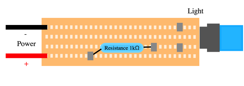
The light from a light-emitting diode, LED for short, can be viewed by the human eye as monochromatic. This means it appears to only light up as one color. From theory we know that a LED cannot be monochromatic, thus proving one of the biggest differences between a LED and a laser. More importantly, the light from a LED is not coherent, meaning that the light waves do not have the same frequency. A LED loses little energy to heat as it applies most of its energy to light up the diode. This is a very useful property.
To create a simple LED-circuit you only need a couple of components: a LED, a resistance, some wires, a circuit board and a voltage source.
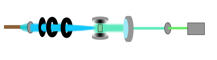
As one can see in the figure, our setup contains the following components: a LED-circuit as light source, lenses, two color filters, two mirrors, a spectrometer and a CCD-camera. The purpose of the lenses is to focus the light from the LED-circuit into a thin beam. This will make the LED-light more similar to a laser, and also increase the intensity of the light by concentrating it into a smaller radius. In order to make our light source act more like a laser, we need the light to have monochromatic properties. By using a blue color filter we can remove some of its spectrum, and obtain a correct wavelength for the GFP and yeast. It is worth mentioning that even though we use filters and lenses to focus the light, we still have to keep the LED at a maximum of 20V and hopefully the intensity is high enough for lasing to happen. Ideally, the mirrors we use should be 98% reflective and the last 2% should be emitted light that we can detect. We were not able to acquire mirrors of that sort, which is why our setup looks a bit different from that of a regular laser. The solution (both GFP or yeast) will be placed between the mirrors, in order to increase the effect of the light emitted from the solution. To be able to gather the light emitted from the GFP, which will be emitted in all directions, we place a big lense next to the mirror chamber. This lense will focus the light from the solution into a filter that removes the wavelengths that belongs to the LED, and by that we obtain the wavelengths we want to observe in a spectrometer or CCD-camera.
To be able to separate the fluoresence and the lasing with our setup we need to look at the spectre of the light waves emitted from the solution we are working with. The spectre of GFP is a broad peak as opposed to the laser, which has only one clear peak. When looking at our spectre we need to look for the clear peak, the laser peak. This will prove that we have succeeded in making the proteins lase, which will hopefully result in us proving the concept of a biolaser.
Our CCD-camera do not have a lense, only a detector in place. In order to know if we will get an image we can see and work with, we need to calculate how big the detected image potentially will be. We are working with wavelengths that go roughly from 505 nm-515 nm, so we wish to calculate the angle between the two waves when they pass through the slit of the spectrometre. We also know that 4000 bars occupy a space of 2.5 cm, so we can calculate \(d\):
Our CCD-camera do not have a lense, only a detector in place. In order to know if we will get an image we can see and work with, we need to calculate how big the detected image potentially will be. We are working with wavelengths that go roughly from 505 nm-515 nm, so we wish to calculate the angle between the two waves when they pass through the slit of the spectrometre. We also know that 4000 bars occupy a space of 2.5 cm, so we can calculate \(d\):
\begin{align}
d = 2.5 \cdot 10^{-3} / 4000 = 6.25 \cdot 10^{-6} m \\
\theta = sin^{-1} \left(\frac{505 \cdot 10^{-9}m}{6.25 \cdot 10^{-6}m}\right) = 0.081 rad \\
\phi = sin^{-1} \left(\frac{515 \cdot 10^{-9} m}{6.25 \cdot 10^{-3}}\right) = 0.082 rad
\end{align}
The distance from the grid to the tip of the spectrometre (where we would out our camera) is 0.3m. So, the space between the two waves (and so, the size of our image) is:
\begin{align}
(0.082 - 0.081) \cdot 0.3m = 0.3mm
\end{align}
It is also worth mentioning that the angle at which the waves pass through the grid is more or less 5 degrees. To check if this works with our camera, we take the number of pixels pr 5 mm, and get:
\begin{align}
\frac{0.005 m}{750 px} = 6.67 \cdot 10^{-6} = 7 \mu m
\end{align}
Anything bigger than 7 \(\mu \) m should be easily observed, and our image should project at around 0.3 mm, so we are good to go! This is where the spectrometre and the CCD camera come into play. By knowing more or less the angle at which the spectre will be emitted we can place the camera where the spectre is sure to appear, and get a good measure of the spectre on screen.