| Line 3: | Line 3: | ||
{{:Team:SUSTech_Shenzhen/nav}} | {{:Team:SUSTech_Shenzhen/nav}} | ||
{{:Team:SUSTech Shenzhen/templates/page-header-model| | {{:Team:SUSTech Shenzhen/templates/page-header-model| | ||
| − | url=wiki/images/1/17/T--SUSTech_Shenzhen--Model.svg|size=100px|title=Worms | + | url=wiki/images/1/17/T--SUSTech_Shenzhen--Model.svg|size=100px|title=Worms Locmotion|subtitle=Model}} |
{{:Team:SUSTech_Shenzhen/main-content-begin}} | {{:Team:SUSTech_Shenzhen/main-content-begin}} | ||
| Line 15: | Line 15: | ||
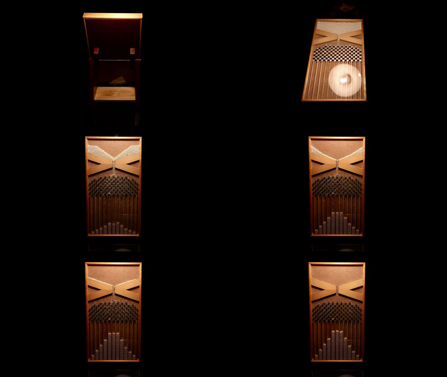
{{SUSTech_Image_Center_8 | filename=T--SUSTech_Shenzhen--Microfuildics--gerdun.gif | caption=<B>Fig. 1 The simulation of Galton board </B>}} | {{SUSTech_Image_Center_8 | filename=T--SUSTech_Shenzhen--Microfuildics--gerdun.gif | caption=<B>Fig. 1 The simulation of Galton board </B>}} | ||
| − | Details: | + | ==Details:== |
Gaussian distribution is very common in nature and important in statistics. This distribution is tied to many natural phenomena. In our experiment, we use Gaussian plate to see C.elegans’ distribution. Then we use it to see the change of C.elegans’ distribution after adding attraction or repellent factor(Fig.2). | Gaussian distribution is very common in nature and important in statistics. This distribution is tied to many natural phenomena. In our experiment, we use Gaussian plate to see C.elegans’ distribution. Then we use it to see the change of C.elegans’ distribution after adding attraction or repellent factor(Fig.2). | ||
| Line 21: | Line 21: | ||
{{SUSTech_Image_Center_fill-width | filename=T--SUSTech_Shenzhen--Microfluidics--fig5.png |width=1000px| caption=<B>Fig. 2 The Gaussian distribution A)</B> The ideal Gaussian distribution before adding chemicals. <B> B) </B>The changed Gaussian distribution after adding chemicals by using the first diffusion methods, which means diacetyl diffuse in the same plate as the Gaussian chip.}} | {{SUSTech_Image_Center_fill-width | filename=T--SUSTech_Shenzhen--Microfluidics--fig5.png |width=1000px| caption=<B>Fig. 2 The Gaussian distribution A)</B> The ideal Gaussian distribution before adding chemicals. <B> B) </B>The changed Gaussian distribution after adding chemicals by using the first diffusion methods, which means diacetyl diffuse in the same plate as the Gaussian chip.}} | ||
| − | Firstly, we introduced a parameter | + | Firstly, we introduced a parameter ‘k<sub>a</sub>’ (0<=k_a<=1) to describe how much the previous choice influences the current choice (Fig.3 缺). |
The ‘k<sub>a</sub>’ is defined as the absolute value of the difference between the probability of two direction choices(Fig.4 缺). | The ‘k<sub>a</sub>’ is defined as the absolute value of the difference between the probability of two direction choices(Fig.4 缺). | ||
| + | It means the greater the ‘k<sub>a</sub>’ is the greater the influence of previous choice is. Especially, when ‘k_a’ is zero, the simulation model is more like Gaussian distribution. | ||
| + | We counted the number of C.elegans in each channel and calculated the parameter ‘k<sub>a</sub>’ at first(Fig.5). | ||
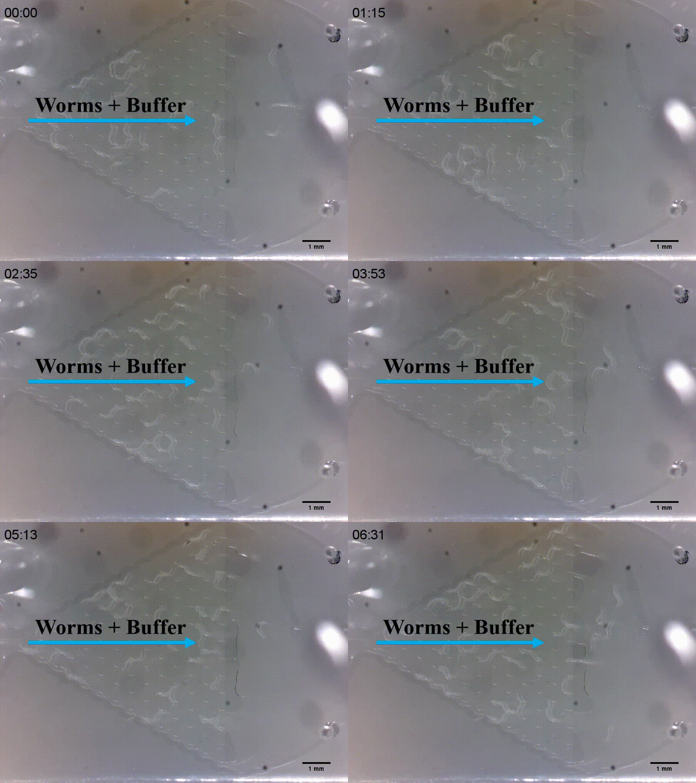
| − | + | {{SUSTech_Image_Center_8 | filename=T--SUSTech_Shenzhen--3.gif | caption=<B>Fig. 5 Gaussian plate to study locomotion on-chip</B>}} | |
| − | + | ||
| − | + | ||
| − | + | ||
| − | + | ||
| − | + | ||
| − | + | ||
| − | + | ||
| − | + | ||
| − | + | ||
| − | + | ||
| − | + | ||
| − | + | ||
{|class="table table-striped" | {|class="table table-striped" | ||
| Line 58: | Line 48: | ||
{{SUSTech_Shenzhen/bmath|equ=<nowiki> k=\frac{same turning-different turning}{total turning}=\frac{(20+10-12-9)}{(20+10+12+9)}=0.18</nowiki>}} | {{SUSTech_Shenzhen/bmath|equ=<nowiki> k=\frac{same turning-different turning}{total turning}=\frac{(20+10-12-9)}{(20+10+12+9)}=0.18</nowiki>}} | ||
| + | Assume that ‘k_a’ doesn’t change when we add attraction or repellent factors. Then this model can be used to stimulate C.elegans preference considering ‘k_a’. | ||
| + | |||
| + | We can analyze how much the factor attracts or repels the C.elegans by introducing another parameter ‘k_perf’ (0<=k_perf<=1). | ||
| + | |||
| + | Both parameters set above are dependent on the assumption that parameters values are proportional to the probability they affect the C.elegans’ choice. | ||
| + | |||
| + | For example, if ‘k_a’ equates to ‘0’, previous choice doesn’t affect current choice at all. If ‘k’ equates to ‘1’, the worm’s next choice is totally determined by the previous choice. Final result will show poly distribution(C.elegans will only pass through the rightmost or leftmost channels). When ‘k’ equates to 0.5, a worm has 25% probability of turning right/left and 75% probability of turning left/right at a crossing. ‘k_perf’ (attraction or repellent parameter) is the same as ‘k_a’. | ||
| + | |||
| + | ==Result:== | ||
| + | |||
| + | Simulation results are shown in two steps: | ||
| + | 1.Determining ‘k_a’: To determine ‘k_a’, we did a experiment without adding factors‘k_a’ equates to 0.18, according to the table shown above. | ||
| + | 2. a. Compare Stimulated 100000 worms with experimental data. | ||
| − | {{SUSTech_Image_Center_8 | filename=T--SUSTech_Shenzhen-- | + | {{SUSTech_Image_Center_8 | filename=T--SUSTech_Shenzhen--Locomotion_Model1-.png|width=6000px|caption=<B></B>}} |
| − | {{ | + | {{SUSTech_Image_Center_fill-width | filename=T--SUSTech_Shenzhen--Locomotion_Model2-.png|width=6000px|caption=<B></B>}} |
| − | {{SUSTech_Image_Center_8 | filename=T--SUSTech_Shenzhen-- | + | {{SUSTech_Image_Center_8 | filename=T--SUSTech_Shenzhen--Locomotion_Model3-.png|width=6000px|caption=<B></B>}} |
| − | {{ | + | {{SUSTech_Image_Center_fill-width | filename=T--SUSTech_Shenzhen--Locomotion_Model4-.png|width=6000px|caption=<B></B>}} |
Revision as of 12:41, 28 October 2017
Worms Locmotion
Model
Contents
This model describes how microfluidics Gaussian distribution plate works when we use this device to test C.elegans’ preference in the plate.If the plate works, the model can further describe how much preference the C.elegans show when attraction or repellent factor is added.
Different from classical Galton board(Fig.1), it is worms rather than balls running on the plate. We use worms as the “ball”. However, when a worm is choosing a direction at the crossing, its previous choice may influence current choice due to worm’s relative long body.
Details:
Gaussian distribution is very common in nature and important in statistics. This distribution is tied to many natural phenomena. In our experiment, we use Gaussian plate to see C.elegans’ distribution. Then we use it to see the change of C.elegans’ distribution after adding attraction or repellent factor(Fig.2).
Firstly, we introduced a parameter ‘ka’ (0<=k_a<=1) to describe how much the previous choice influences the current choice (Fig.3 缺).
The ‘ka’ is defined as the absolute value of the difference between the probability of two direction choices(Fig.4 缺).
It means the greater the ‘ka’ is the greater the influence of previous choice is. Especially, when ‘k_a’ is zero, the simulation model is more like Gaussian distribution.
We counted the number of C.elegans in each channel and calculated the parameter ‘ka’ at first(Fig.5).
| Count | Firstly Turn Left | Firstly Turn Right |
| Secondly Turn Left | 20 | 9 |
| Secondly Turn Right | 12 | 10 |
k=\frac{same turning-different turning}{total turning}=\frac{(20+10-12-9)}{(20+10+12+9)}=0.18
Assume that ‘k_a’ doesn’t change when we add attraction or repellent factors. Then this model can be used to stimulate C.elegans preference considering ‘k_a’.
We can analyze how much the factor attracts or repels the C.elegans by introducing another parameter ‘k_perf’ (0<=k_perf<=1).
Both parameters set above are dependent on the assumption that parameters values are proportional to the probability they affect the C.elegans’ choice.
For example, if ‘k_a’ equates to ‘0’, previous choice doesn’t affect current choice at all. If ‘k’ equates to ‘1’, the worm’s next choice is totally determined by the previous choice. Final result will show poly distribution(C.elegans will only pass through the rightmost or leftmost channels). When ‘k’ equates to 0.5, a worm has 25% probability of turning right/left and 75% probability of turning left/right at a crossing. ‘k_perf’ (attraction or repellent parameter) is the same as ‘k_a’.
Result:
Simulation results are shown in two steps:
1.Determining ‘k_a’: To determine ‘k_a’, we did a experiment without adding factors‘k_a’ equates to 0.18, according to the table shown above.
2. a. Compare Stimulated 100000 worms with experimental data.


