Team:York/Results
Our Results
Detailed, below, are the results we obtained during the various experimental stages of this project. Accompanying each display of data is a small paragraph of conclusive remarks which aims to outline the importance or significance of the results.
You can get straight to a section by following these links:
- Modifying Chlamydomonas reinhardtii
- Growth Tests
- Constructs
- Size and Shape Analysis
- Cell Density Analysis
- Motility Observations
- Conclusions
Modifying C. reinhardtii
We attempted to introduce MEX-1, a maltose exporter gene normally found in the plastid membrane, into the cell membrane of C. reinhardtii.
Unfortunately, the results were bleak.
The GC-content of C. reinhardtii’s genome is around 60% [1]. This is a likely cause of the modification’s failure, since high GC content is linked with difficulty in amplifying through PCR [2].
Further, despite our best attempts at performing the transformation, we simply did not have enough time to get a successful result. C. reinhardtii has a relatively slow growth rate (doubling around once every 8 hours at 25°C [3]) which, coupled with the waiting time for sequencing results, meant that, over the short period in which we could use laboratories in our Department of Biology, we only had time for two attempts at modification. Both were unsuccessful and, thence, we had to abandon the idea that C. reinhardtii could export maltose as a carbon source for LW06.
Will it grow, if...?
Concurrently with the above, we tested the growth of our organisms under different circumstances and on different media to see what ramifications the effects would have for our proposed co-culture.
LW06 on Maltose

- Figure 1: Maltose test plate 1 box plot. Plate 1 has serious anomalies in the blanks and controls when compared to plates 2 and 3. RV on y axis is the regression values. Results from this experiment where discounted due to problems with the control and blank samples.

- Figure 2: Maltose test plate 2 box plot. Missing data points in the blanks and controls are due to OD data not being high enough to be logged by R studio software. RV on y axis is the regression values.

- Figure 3: Maltose test plate 3 box plot. RV on y axis is the regression values.

- Figure 4: Maltose test plate 1 column graph, mean growth rates on maltose gradient in 96 well plates. Media maltose (1-8) represents columns 5–12 (TP.Maltose) wells. Given previously described issues with controls data from this experiment is not to be used for analysis.

- Figure 5: Maltose test plate 2 column graphs, mean growth rates on maltose gradient in 96 well plates. Media maltose (1-8) represents columns 5–12 (TP.Maltose) wells.

- Figure 6: Maltose plate 3 column graph, mean growth rates on maltose gradient in 96 well plates. Media maltose (1-8) represents columns 5–12 (TP.Maltose) wells.
Results: Consistency is shown for high growth in column 5 (1g/L) but remains more or less level throughout the increasing maltose concentrations. Such consistency indicates LW06 is somewhat poor at maltose metabolism but is able to survive on it. Mean growth rates are small, though this is potentially explained by a highly limiting culture volume. However, data from the plate reader indicates clear exponential and plateau events during growth. In conclusion, growth under maltose conditions is possible. Conditioning for maltose consumption may be required to improve final culturing with C. reinhardtii when it is exporting maltose, in future co-cultures. The problems with the first experimental run, contamination in the blanks and controls, were most likely due to condensation on the interior lid or displacement of culture material in the controls and blank sections of the plate during agitation. As a result of this, data from this experiment is to be discounted for analysis and should be considered when proceeding with experiments in the future as to avoid issues of contamination.
LW06 on Home Blend Medium

- Figure 7: Home blend (Hblend) test plate 1. Regression values (y axis) show that TP-Maltose performs worse than TP-Glucose. Hblend-Glucose greatly out performs Hblend-Maltose, but is comparable to TP-Maltose.

- Figure 8: Hblend test plate 1. Mean growth rates here show that the growth rate for Hblend-Glucose is much greater than TP or Hblend-Maltose. TP-Maltose outperforms our Home blend recipe.
- A T-test was conducted for TP.Maltose and Hblend.Maltose. T-test (Degrees of Freedom = 48, p = 8.82 x 10⁻¹⁰). This indicates significant difference between media types.

- Figure 9: Hblend test plate 2. Regression values (y axis), as in figure 7, show that TP and Hblend-Maltose are out performed by Hblend-Glucose.

- Figure 10: Hblend test plate 2. Mean growth rates here show Hblend-Glucose out performs TP or Hblend-Maltose with no difference between the latter pair in terms of growth.
- A T-test was conducted for the second plate. T-test (D.o.F. = 48, p = 0.058255). For the second plate, no statistical significance between media types was indicated.
Results: Overall, Hblend performs unremarkably when compared to TP media. Despite having much higher micronutrients, Hblend does not perform as well as we hypothesised. Some data collected indicates that a longer run time may have had an effect, but it is unlikely that this would lead to major improvements over the TP media. The problem seems to be the uptake or metabolism of maltose. Conditioning our organisms to grow on maltose may improve growth rates in a co-culture. However, such a limitation may work to the advantage of the co-culture. A key problem to consider was the greatly divergent growth rates between C. reinhardtii and the LW06 E. coli strain. This reduced growth with maltose as the carbon source may provide a sufficient rate limiter on the growth of LW06 to avoid complete culture saturation with the E. coli in future co-cultures.
C. reinhardtii Ethanol Tolerance

- Figure 11: Cell counts for C. reinhardtii via multiple well plate readers. Readings taken ~24hours manually.

- Figure 12: Cell counts for C. reinhardtii via multiple well plate readers. Readings taken ~24hours manually.
Results: C. reinhardtii is able to tolerate an increase of ethanol to at the most 3.2% (as a portion of media). Given rates of increase it seems that it could tolerate much higher concentrations. This is encouraging, as ethanol resistance of the C. reinhardtii would likely be sufficient to survive upper limits of the LW06 strain’s ethanol production. Interestingly, C. reinhardtii experiences better growth at higher concentrations of ethanol, there is not a clear reason this is the case. Addition of ethanol to the media may have made growth conditions more amenable to C. reinhardtii. There is some chance that the ethanol may have evaporated which, while possible, is unlikely due to the sealing of the plate. Overall, it seems that C. reinhardtii would be able to survive the proposed amount of ethanol that could be produced by the LW06.
Co-culture of C. reinhardtii and E. coli LW06
There's a large growth disparity between the two organisms [3][4], so we also performed an experiment to check if LW06 would vastly outperform C. reinhardtii on all types of media.
Growth in a Co-culture

- Figure 13: Cell counts for LW06 in each culture via spread plating at 104 dilutions.

- Figure 14: Cell counts for C. reinhardtii via manual haemocytometer microscope cell counting at a 104 dilution.

- Figure 15: Overlaid cell counts for the co-culture. LW06 represented by blue points and C. reinhardtii by orange.
Results: Overall LW06 outperforms C. reinhardtii in all but one of the cultures (Tube 4). It is encouraging to see LW06 perform well on TP.Maltose and TAP.Maltose, although the latter may have been due to the presence of a second carbon source in the form of acetate. It is odd that in every one of the experiments tube that were inoculated with 100 μl of 0.5-1.0 OD LW06 that the cell counts are considerably lower. It seems that the initial starting cell density may have inhibited growth but it is not clear why this effect would continue when dispersed in the co-culture. Alternatively, an unknown error may have occurred at some point during inoculation. From the results it is clear that, if it was some unknown or unnoticed error, it was made consistently in every one of the co-cultures with 100 μL inoculation. No relevant conclusions can be drawn from this. However, considerations such as the growth limiting factor of the TP.Maltose may work in our interest as to avoid culture saturation with LW06.
An obvious error, in hindsight, is the issue of the 10 μL inoculation. It is likely that a much higher volume added to the culture would have improved the results. This would have provided a high enough cell density, should growth have not be great enough during co-culturing with the modified C. reinhardtii in TP media. Overall co-cultures with these two organisms are possible, but higher OD/volume of inoculant may be needed.
Constructs
We constructed several plasmids to attempt the introduction of MEX-1 into the outer membrane of C. reinhardtii. The figures, below, show maps of these plasmids and our evidence that we correctly made the constructs.
Plasmid Maps
Results: We used plasmid pLM005 as our vector (see figure 16), which is designed specifically for the expression of eukaryotic ORFs and incorporates a YFP fusion at the C terminal end of the recombinant protein, so we could detect localisation of our edited MEX-1 to the outer membrane.
Cutting of the plasmid at the two HpaI sites removes a small fragment of the plasmid and provides the insertion site for the recombinant gene. Once amplified, the vector is cut again at the eco-RV sites (not shown) to produce a cassette for transformation directly into the C. reinhardtii genome.
We successfully cloned and inserted the MEX-1 gene into the pLM005 vector (see figure 17, gel electrophoresis and fluorescent microscopy images below). Our strategy for relocation of MEX-1 (which is a chloroplast membrane protein [5]) was to remove the signal peptide of MEX-1 by PCR cloning and assemble the truncated MEX-1 gene with the signal peptide sequence of known outer membrane protein ACA3 (see figure 18). We were able to successfully assemble this construct (see gel electrophoresis), however we did not manage to successfully transform it into C. reinhardtii.
BioBrick
Results: We designed a biobrick based on the pLM005 plasmid which we used for our project (described above). It uses the silver RFC[23] prefix and suffix for insertion of a eukaryotic ORF into that site where it is tagged at the C terminal end by a YFP and expression is driven by the strong, constitutive PsaD promoter (see figure 19). We used the complimentary 1000bp gblock offer from IDT to synthesise fragments of our biobrick with 18bp overlaps for Gibson assembly. However, this large construct required 7 fragments (see figure 20) and we were unsuccessful in our attempts to assemble.
Evidence

- A: Gel electrophoresis of PCR cloned genes from plasmid library of C. reinhardtii genome. ACA3 TMD is the region of the ACA3 gene 5' of the first transmembrane domain, ACA3 SP is the region of the ACA3 gene predicted to code the signal peptide.

- B: Gel electrophoresis of PstI digested MEX-1 plasmids after Hifi assembly. Colonies 1,3,4,6 &10 appear to contain successfully assembled constructs.
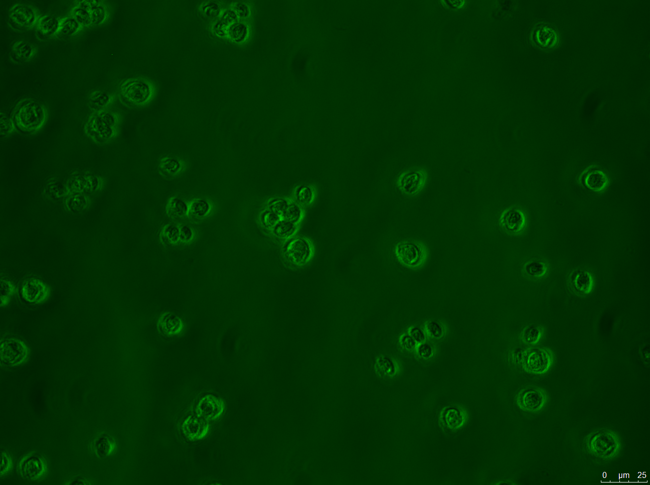
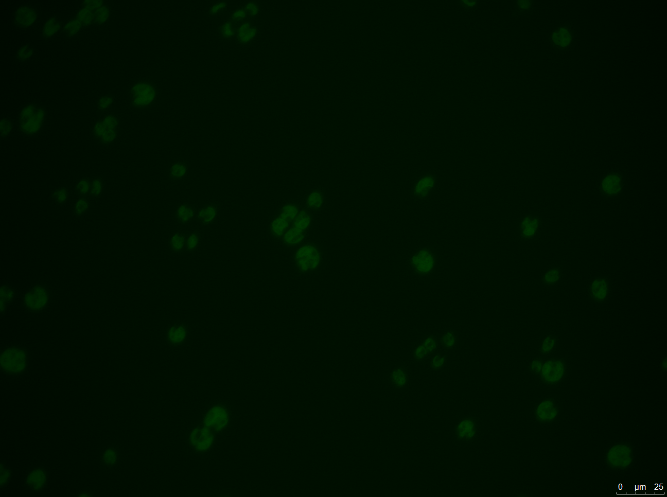
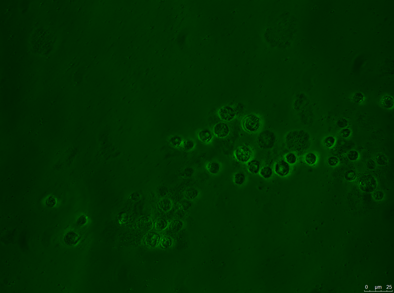
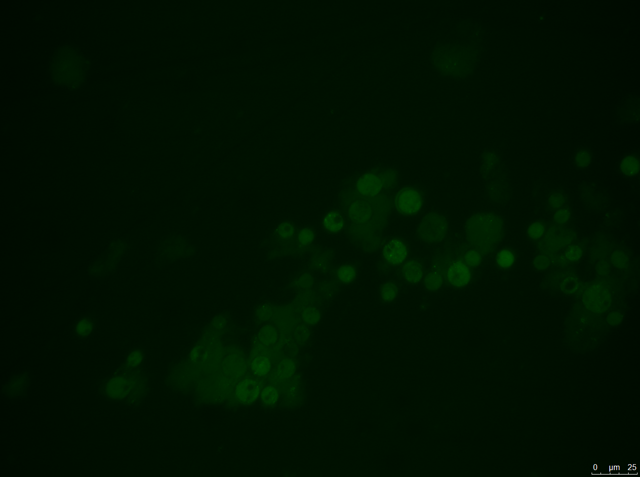
- A: Wild-type Chlamydomonas reinhardtii under a fluorescence microscope before filtering for the Venus fluorescence wavelength.
- B: The wild-type under fluorescence microscope with a filter for the Venus fluorescence wavelength.
- C: C. reinhardtii after our insertion of the Venus tag, before wavelength filtering.
- D: C. reinhardtii after our insertion of the Venus tag, after wavelength filtering.
Results: Figure 22 shows our gel electrophoresis data, confirming that we correctly assembled our construct. Figure 23 shows that we were able to insert our Venus control into C. reinhardtii. Unfortunately, the same was not true of our MEX-1 construct.
Size and Shape Analysis
Though we had some trouble with alignment of lenses, we achieved several results wherein observing the shape of an organism in the focal plane was facilitated. We present the results below. Organisms are outlined in red boxes.
Confirming Shapes and Sizes of Organisms

- Figure 24: E. coli strain BW25113. Its size is (6 x 4) pixels. This corresponds to (1.34 x 0.90) µm.

- Figure 25: E. coli strain BW25113. Its size is (9 x 6) pixels. This corresponds to (2.02 x 1.34) µm.

- Figure 26: This sample contained wildtype E. coli and C. reinhardtii. It was provided by Dr. Laurence Wilson, captured using his own DIHM. The hologram was produced using our software and the size of E. coli was (6 x 4) pixels, which equates to (1.34 x 0.90) µm.

- Figure 27: Chlamydomonas reinhardtii. The sizes were as follows. A: (9 x 10) pixels, (10.1 x 11.2) µm. B: (9 x 9) pixels, (10.1 x 10.1) µm. C: (10 x 9) pixels, (11.2 x 10.1) µm. D: (10 x 9) pixels, (11.2 x 10.1) µm.
Results: These results show that our software is capable of producing holograms within which the shapes of organisms can be distinguished. In figures 24 to 26, the E. coli can be seen to be rod shaped, approximately 2 µm in one direction and 1 µm in the other, as expected [6]. In the figure 27, C. reinhardtii is approximately circular with diameter around 10 µm, also as expected [3]. These are promising results which show the potential for the technique to be used to distinguish between organisms within a co-culture, especially when there is a size discrepancy. This is exemplified in figure 26, most of all. Figures 24, 25 and 27 are also evidence that the quality of images taken with our hardware is sufficient for shape detection. As seen here, we also tested the ability to find the size and shape of organisms with Saccharomyces cerevisiae, which is of an intermediate size when compared with E. coli and C. reinhardtii. The S. cerevisiae was kindly provided by the iGEM Aachen 2017 team.
Cell Density Analysis
We used our analysis software to count the cells in manually-selected focal planes. All of the below images are from data taken with our own hardware and software. We then calculated the volume of the hologram in each case (accounting for magnification, step size and number of steps) and used both to find the number of cells per millilitre. We used the formula: Cells/mL = (D x C x 10-6) / (5122 x N x ((1.12/M)x10-6)3 ); wherein C is the counted number of blobs from the analysis software, D is the dilution number compared with the corroborated sample (e.g. D = 100 for a 1 part in 100 dilution, D = 1 for an undiluted sample), M is the magnification and N is the number of steps between the focal plane being analysed and the closest other plane with focused cells. In most cases N was 150, indicating the whole hologram had only one focused section. We corroborated our values' relevance by comparing to either an optical density reading or a reading from a ThermoFisher Countess II FL Automated Cell Counter.
Confirming Cell Counts

- Figure 28: C. reinhardtii: C = 13, D = 10, M = 1, N = 150. The Countess II FL gave a reading of (5.19 x 10⁶) cells/mL. Our calculated value was (2.4 x 10⁶) cells/mL.

- Figure 29: C. reinhardtii: C = 113, D = 1, M = 5, N = 150. The Countess II FL gave a reading of (2.03 x 10⁸) cells/mL. Our calculated value was (2.6 x 10⁸) cells/mL.

- Figure 30: TAP medium only: C = 10, D = 1, M = 1, N = 150. There are no microorganisms present, the diffraction patterns here are due to dust on the slide. The Countess II FL gave a reading of (1.47 x 10⁴) cells/mL. Our calculated value was (1.8 x 10⁵) cells/mL.

- Figure 31: E. coli: C = 10, D = 100, M = 5, N = 150. The foci were slightly misshapen (but still countable) due to misalignment of the lens during setup. The OD reading returned (4 x 10⁹) cells/mL. Our calculated value was (2.3 x 10⁹) cells/mL.

- Figure 32: Galdieria sulphuraria: C = 248, D = 1, M = 1, N = 150. The Countess II FL reading returned (5.3 x 10⁶) cells/mL. Our calculated value was (4.5 x 10⁶) cells/mL.
Results: Figure 28 shows a well focused, not-magnified image of C. reinhardtii. It is clear from the image that several cells that were present within the area of the image were not detected. However, many, if not all, of them did not pass through the focus of the constructed hologram. Further, the cell count we obtained was only a factor of 2 different to that given by an lab-grade automated cell counter. Considering the minimally developed analysis software, this is a promising achievement that could likely be improved with time and better algorithms.
Figure 29 shows a 5x magnified image of C. reinhardtii. The diffraction patterns are misshapen (we expect circles, like in figure 28, but larger). This is due to the lens being slightly misaligned, which points to a weakness of the hardware's design. Perfect alignment is difficult to achieve when the levelness of component platforms must be adjusted by hand. It can be seen, from the figure, that some of the detected blobs are in erroneous positions and that some cells remain undetected. Upon counting manually, it seems that these two errors roughly cancel each other out. We conclude from this figure that the design of the hardware and software must be improved before industrial use is realisable, though this (and our other data) serve as proof of concept.
Figure 30 shows a not-magnified image of a slide whose contents is solely TAP medium. The diffraction patterns that are apparent are most likely caused by dust or imperfections in the slide. The count we obtained for this hologram was an order of magnitude higher than the equivalent result from the automated cell counter, but was an order of magnitude (or more) lower than that for other not-magnified holograms that we took, even the least populous. The conditions used for detection in this image were the same as for figure 28, showing that our uncertainty in a measurement like this is likely around 10%. This is twice that of the automated cell counter we used [7]. This is a positive result, as it implies that, as the analysis techniques we have used are developed in future, we can approach the accuracy of widely used lab equipment.
Figure 31 shows E. coli LW06 at 5x magnification. The cells' diffraction patterns were misshapen for the same reasons as those presented, above, for figure 29. Regardless, the count achieved was around a factor of 2 less than the value obtained through optical density analysis (which was performed at 600 nm wavelength). Yet again, as evidence that our concept is useful, this result is promising.
Figure 32 shows Galdieria sulphuraria at 1x magnification. This was a densely populated sample, though the software still performed well. The blue outline denotes that the cell was detected by looking at the gradient image. The percentage difference between the Countess II FL reading and our own value was 15%. This equates to a difference in count of around 7. This serves as perhaps our best evidence that, when all goes according to plan with our current hardware and software, it functions as an at least somewhat viable alternative to other cell counting methods.
Confirming Cell Counts in a Co-Sample

- Figure 33: C. reinhardtii and G. sulphuraria: C = 21, D = 1, M = 1, N = 150. The Countess II FL reading returned (6.28 x 10⁵) cells/mL for the combined total of the organisms. Our calculated value was (3.8 x 10⁵) cells/mL.

- Figure 34: C. reinhardtii and G. sulphuraria: C = 9, D = 1, M = 1, N = 150. The Countess II FL was only capable of reading the total cell count, so we have no corroboratory datum for this test. Our count for the larger species was (1.6 x 10⁵) cells/mL.
Results: Figures 33 and 34 show a co-sample of C. reinhardtii and G. sulphuraria. It was made by combining a sample of a set volume for each of the organisms. The C. reinhardtii sample had (4.17 x 10⁵) cells/mL and the G. sulphuraria had (3.02 x 10⁵) cells/mL. We suppose, therefore, that Galdieria made up 42.0% of the resultant co-sample's organisms by number. Our count from figure 34 is 42.1% of the count in figure 33. Figure 33's count was found by considering the entire range of documented radii for both organisms [7][8]. Figure 34's count was the upper half of that range, within which G. sulphuraria has been documented to reach during its lifecycle [8]. We conclude that it is most likely that we have found the ratio between two organisms of slightly different size in a co-sample. This, we present as evidence that our microscope and software are a useful tool for the determination of cell density in samples containing multiple visibly distinguishable organisms.
In short, the above data evidences the promising potential of our software and hardware combination with respect to use as a non-intrusive and fast method of monitoring the growth of cells in monocultures and in co-cultures. All of the image processing and calculations as outlined above can be done, in minutes, on the same Raspberry Pi that is used to take the images.
Motility Observations
Below we present evidence that our microscope is capable of showing the movement of organisms. Unfortunately, C. reinhardtii was the only organism we captured moving autonomously. We also tried to modify E. coli to increase its motility (see the Description page), though this was unsuccessful. We borrowed another strain (DB5) that moves a lot, too. When we tried to look at it using our microscope, we couldn't see any moving cells, despite being able to see them under a light microscope. We did capture footage of E. coli moving due to the flow of liquid medium, however. It is presented below, also.
Chlamydomonas reinhardtii Moving in Samples

- Figure 35: A GIF of a C. reinhardtii cell moving in a sample at 5x magnification.
- Figure 36: A video showing a C. reinhardtii cell moving in a sample at 5x magnification.
Results: It is apparent that the cells, above, are moving autonomously when compared with the motion due to flow as seen for E. coli below. The movement of C. reinhardtii is considerably more erratic and does not follow a single line/smooth path.
E. coli DB5 Drifting with Flow of Medium
- Figure 37: A video showing E. coli cells moving, from the top-right in a down/left direction, in a sample at 5x magnification.
Results: Though the moving diffraction patterns are faint, it cn be seen that the movement of each cell in the above video is identical, smooth and in a single direction. Hence, we assert that the motion is drift, rather than autonomous transit.
Conclusions
In summary, we can draw several conclusions. We have had some successes and have seen some areas that seem promising but require more work.
The main shortcomings:
- Creating a closed analysis system using a milli-fluidic chamber.
- We came to realise that we required a thinner analysis chamber. Some evidence can be found here.
- Inserting MEX-1 into the outer membrane of Chlamydomonas reinhardtii.
- Our transformation of C. reinhardtii failed. As mentioned here.
- Quantifying the motility of organisms using our DIHM setup.
- We could see C. reinhardtii moving on various occasions, but failed to observe the motility of E. coli DB5, a motile strain. As discussed here.
- Using a UI to control the DIHM from a third party computer.
- We had a great design, there was a compatibility bug that we could not fix in the time we had. As seen here.
The main successes:
- We created inexpensive and functioning upright DIHM hardware and open source holography software.
- The hardware can be seen here. The software is discussed here.
- We created blob detection software which is capable of finding cells of a given size in a focused image.
- The software is mentioned in more detail here.
- We successfully observed the shapes of organisms using our DIHM and holography software.
- This can be seen here.
- We calculated the cell density of samples consistently to a fair degree of accuracy, using our DIHM and holography software.
- As shown here.
- We confirmed that C. reinhardtii and E. coli can grow together in a co-culture.
- This is evidenced here.
- We successfully constructed our MEX-1 plasmid.
- Though we didn't manage to make C. reinhardtii accept it, we present proof that we correctly constructed it here.
Hence, our overarching conclusion is that digital holography is not only low-cost, easily adapted and useful for analysing co-cultures but also holds great potential in terms of future applications. We mention one such future application on our Applied Design page.
References
- [1]: S. Merchant, et al. The Chlamydomonas Genome Reveals the Evolution of Key Animal and Plant Functions, Science
- [2]: Y. Benita, et al. Regionalized GC content of template DNA as a predictor of PCR success, Nucleic Acids Research
- [3]: E. H. Harris, The Chlamydomonas Sourcebook, 2nd Edition
- [4]: A. G. Marr, Growth rate of Escherichia coli, Microbiological Reviews
- [5]: T. Niittylä, A Previously Unknown Maltose Transporter Essential for Starch Degradation in Leaves, Science
- [6]: J. H. Cummings and G. T. Macfarlane, Role of intestinal bacteria in nutrient metabolism, Journal of parenteral and enteral nutrition
- [7]: Countess II FL Automated Cell Counter, ThermoFisher Scientific, as available on 31st October 2017 at www.thermofisher.com/order/catalog/product/AMQAF1000
- [8]: P. Albertano, C. Ciniglia, G. Pinto & A. Pollio, The taxonomic position of Cyanidium, Cyanidioschyzon and Galdieria: an update, Hydrobiologia