Difference between revisions of "Team:York/Description"
Joe McKeown (Talk | contribs) |
Joe McKeown (Talk | contribs) |
||
| Line 94: | Line 94: | ||
<ul style="list-style: none;"> | <ul style="list-style: none;"> | ||
<li><img src="//2017.igem.org/wiki/images/7/7c/IGEM-York-LW06-Maltose-Fig2.png" width=100%"></li> | <li><img src="//2017.igem.org/wiki/images/7/7c/IGEM-York-LW06-Maltose-Fig2.png" width=100%"></li> | ||
| − | <li style="text-align: left; font-size: 14px;"><strong>Figure 2:</strong> Maltose test plate 2 box plot. Missing data points in the blanks and controls are due to OD data not being high enough to be logged by R studio software. RV on y axis is the regression values.<br></li> | + | <li style="text-align: left; font-size: 14px;"><strong>Figure 2:</strong> Maltose test plate 2 box plot. Missing data points in the blanks and controls are due to OD data not being high enough to be logged by R studio software. RV on y axis is the regression values.<br><br></li> |
</ul> | </ul> | ||
</center> | </center> | ||
| Line 113: | Line 113: | ||
<ul style="list-style: none;"> | <ul style="list-style: none;"> | ||
<li><img src="//2017.igem.org/wiki/images/1/10/IGEM-York-LW06-Maltose-Fig4.png" width="100%"></li> | <li><img src="//2017.igem.org/wiki/images/1/10/IGEM-York-LW06-Maltose-Fig4.png" width="100%"></li> | ||
| − | <li style="text-align: left; font-size: 14px;"><strong>Figure 4:</strong> Maltose test plate 1 column graph, mean growth rates on maltose gradient in 96 well plates. Media maltose (1-8) represents columns 5 – 12 (TP.Maltose) wells. Given previously described issues with controls data from this experiment is not to be used for analysis.</li> | + | <li style="text-align: left; font-size: 14px;"><br><strong>Figure 4:</strong> Maltose test plate 1 column graph, mean growth rates on maltose gradient in 96 well plates. Media maltose (1-8) represents columns 5 – 12 (TP.Maltose) wells. Given previously described issues with controls data from this experiment is not to be used for analysis.</li> |
</ul> | </ul> | ||
</center> | </center> | ||
Revision as of 14:38, 16 October 2017
The Project
Upon being asked to find the number of microorganisms in a given sample, the response from members of our iGEM team has invariably been a long sigh and a plea to the realms of the supernatural.
That most human quality - laziness - alongside flaws in traditional techniques, which we will revisit below, has led to us designing a potential solution in the form of a Digital Inline Holographic Microscope (DIHM).
In particular, we discovered that, when studying co-cultures, there are precious few methods of counting cells that are accurate, fast, cheap and non-destructive.
We decided, therefore, to try to bring together two promising areas of science in this project:
Digital Holographic Microscopy and Co-Culturing.
In the Beginning...
When the project began, we had several goals in mind.
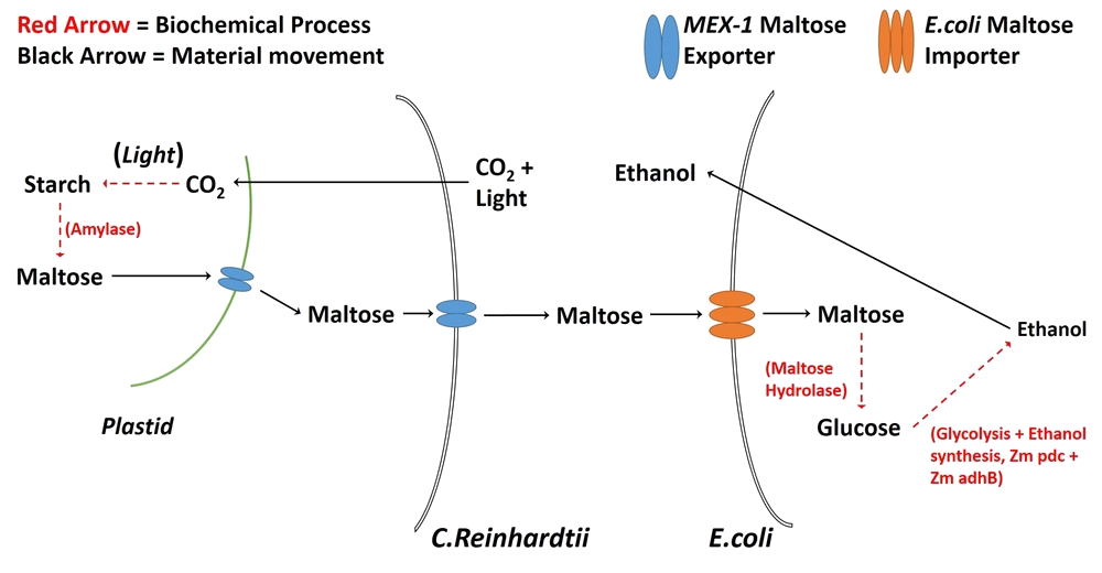
- Modify Chlamydomonas reinhardtii via the MEX-1 gene so that it would export maltose.
- Co-culture the modified C. reinhardtii with Escherichia coli LW06 so that LW06 would render the exported maltose into ethanol.
- Model the growth of both organisms and ethanol production.
- Optimise the production of ethanol in the system by adjusting the ratio of the numbers of each organism.
- Monitor the number of each organism in a closed system via DIHM and milli-fluidic chamber (our QWACC system).
Modifying C. reinhardtii
We attempted to introduce MEX-1, a maltose exporter gene normally found in the plastid membrane, into the cell membrane of C. reinhardtii.
Unfortunately, the results were bleak.
The GC-content of MEX-1 is around 70% (source???) and the GC-content of C. reinhardtii’s genome is around 60% (source???). This is a likely cause of the modification’s failure, since high GC content is linked with difficulty in amplifying through PCR (source???).
Further, despite our best attempts at performing the transformation, we simply did not have enough time to get a successful result. C. reinhardtii has a relatively slow growth rate (doubling around once per week at 25°C (source???)) which, coupled with the waiting time for sequencing results, meant that, over the short period in which we could use laboratories in our Department of Biology, we only had time for two attempts at modification. Both were unsuccessful and, thence, we had to abandon the idea that C. reinhardtii could export maltose as a carbon source for LW06.
Co-culture of C. reinhardtii and E. coli LW06
Concurrently with the above, we tested the growth of both organisms on different media to see which would best support our proposed co-culture.
LW06 on Maltose

- Figure 1: Maltose test plate 1 box plot. Plate 1 has serious anomalies in the blanks and controls when compared to plates 2 and 3. RV on y axis is the regression values. Results from this experiment where discounted due to problems with the control and blank samples.

- Figure 2: Maltose test plate 2 box plot. Missing data points in the blanks and controls are due to OD data not being high enough to be logged by R studio software. RV on y axis is the regression values.

- Figure 3: Maltose test plate 3 box plot. RV on y axis is the regression values.

Figure 4: Maltose test plate 1 column graph, mean growth rates on maltose gradient in 96 well plates. Media maltose (1-8) represents columns 5 – 12 (TP.Maltose) wells. Given previously described issues with controls data from this experiment is not to be used for analysis.

- Figure 5: Maltose test plate 2 column graphs, mean growth rates on maltose gradient in 96 well plates. Media maltose (1-8) represents columns 5–12 (TP.Maltose) wells.

- Figure 6: Maltose plate 3 column graph, mean growth rates on maltose gradient in 96 well plates. Media maltose (1-8) represents columns 5–12 (TP.Maltose) wells.


Digital Inline Holographic Microscopy
Why DIHM?
So, we began the development of an inexpensive DIHM and accompanying software which is able to automatically count cells. Due to the inherently digital nature of this type of microscopy, software can easily be created and adapted such that the DIHM can not only count organisms but, also, differentiate between those that are distinguishable by physical appearance. Among the most important motivators of this hardware/software combination were speed of measurement (our target was the order of seconds or minute per measurement) and low costs for setup and maintenance. Further, in co-cultures wherein neither organism contains a fluorescent marker, the process of counting each type can become a rather complex endeavour. With our QWACC, however, there exists the potential for real-time counting of all physically distinct organisms within a sample.
In the table, below, we have compared several methods of cell counting that are able to distinguish between organisms. This is not quantitative and simply shows how each technique stacks up compared to the rest of those on the list. This is denoted through a traffic light system - green indicates that the method is desirable for the given quality, yellow corresponds to a reasonably desirable quality and red indicates that the technique is undesirable with respect to the quality.

- Table 1: A qualitative comparison of organism counting techniques. Green: desirable; yellow: reasonable; red: undesirable.
In the absence of a DIHM, the technique that we would have most likely used is flow cytometry. This would have been suitable for our needs since, in our modification of Chlamydomonas we inserted a fluorescence gene - Venus "YFP" - and E. coli also fluoresces due to mCherry. This would allow us to count the two organisms by exciting with different wavelengths and measuring the responses. This is a relatively accurate procedure and is not overly time consuming. On the other hand, not every organism is modifiable and therefore it is not always possible to discern the numbers of organisms using this technique. For more thorough comparisons between the techniques specified in the above table, see here.
Limits of QWACC
Experiments in Versatility
Once we had created our QWACC, we wanted to test its capabilities with respect to analysing co-cultures. To do this, we performed several experiments with a variety of co-cultures. The organism combinations were:
- E. coli (ethanol production strain LW06) and C. reinhardtii (strain CC-4533)
- E. coli (ethanol production strain LW06) and E. coli (strain BL21(DE3) with increased motility via parts BBa_K777100 to BBa_K777108)
- Galdieria Sulphuraria (strain currently not known) and E. coli (ethanol production strain LW06)
- Galdieria Sulphuraria (strain currently not known) and C. reinhardtii (strain CC-4533)
A sample of each liquid co-culture was pumped through a milli-fluidic chamber (whose design can be found here) using a peristaltic pump. Then the chamber was positioned over the camera of our QWACC. An image was then taken every few minutes in order to create a hologram. The hologram was then processed into a single PNG containing all the information necessary for counting cells. A blob-detection/circle-detection algorithm was then used to locate and count the cells, with size and shape being used to differentiate between organisms. In the case of co-culture 2 (in the above list), the distinction could not be made via size or shape since both organisms were E. coli and, therefore, physically identical. Instead, we took videos of the co-culture and deciphered, by eye, which were moving faster/more. These, we marked as the E. coli that had been modified to have increased motility. This further tested the versatility of co-culture analysis with the QWACC since it confirms/refutes the possibility that physically identical organisms can also be distinguished through this method.
Results
Co-Cultures
C. reinhardtii and E. coli
The second half of the project involves the creation of a co-culture comprising Escherichia coli and Chlamydomonas reinhardtii. Since E. coli and C. reinhardtii are separated in size by an order of magnitude, it is possible to use so-called blob detection algorithms to locate, count and distinguish between the two organisms in holograms formed by a DIHM.