Team:Heidelberg/Model/Phage Titer
Modeling
Phage Titer
While developing PREDCEL in the lab, we simultaneously developed it in silico so that both sides could benefit from each other. One of the most important parameter of phage assisted directed evolution experiments like PREDCEL and PACE is the phage titer itself. If the phage titer drops washout can occur and the experiment has to be restarted with the disadvantage of loosing library complexity. If the phage titer increases too much, the multiplicity of infection (MOI), that means the amount of phage relative the the amount of E. coli rises too. If fore example the MOI is 10 and an E. coli can only be infected by one phage, nine out of ten phages will not infect an E. coli and thus will not evolve, but still make up most of the phage population.
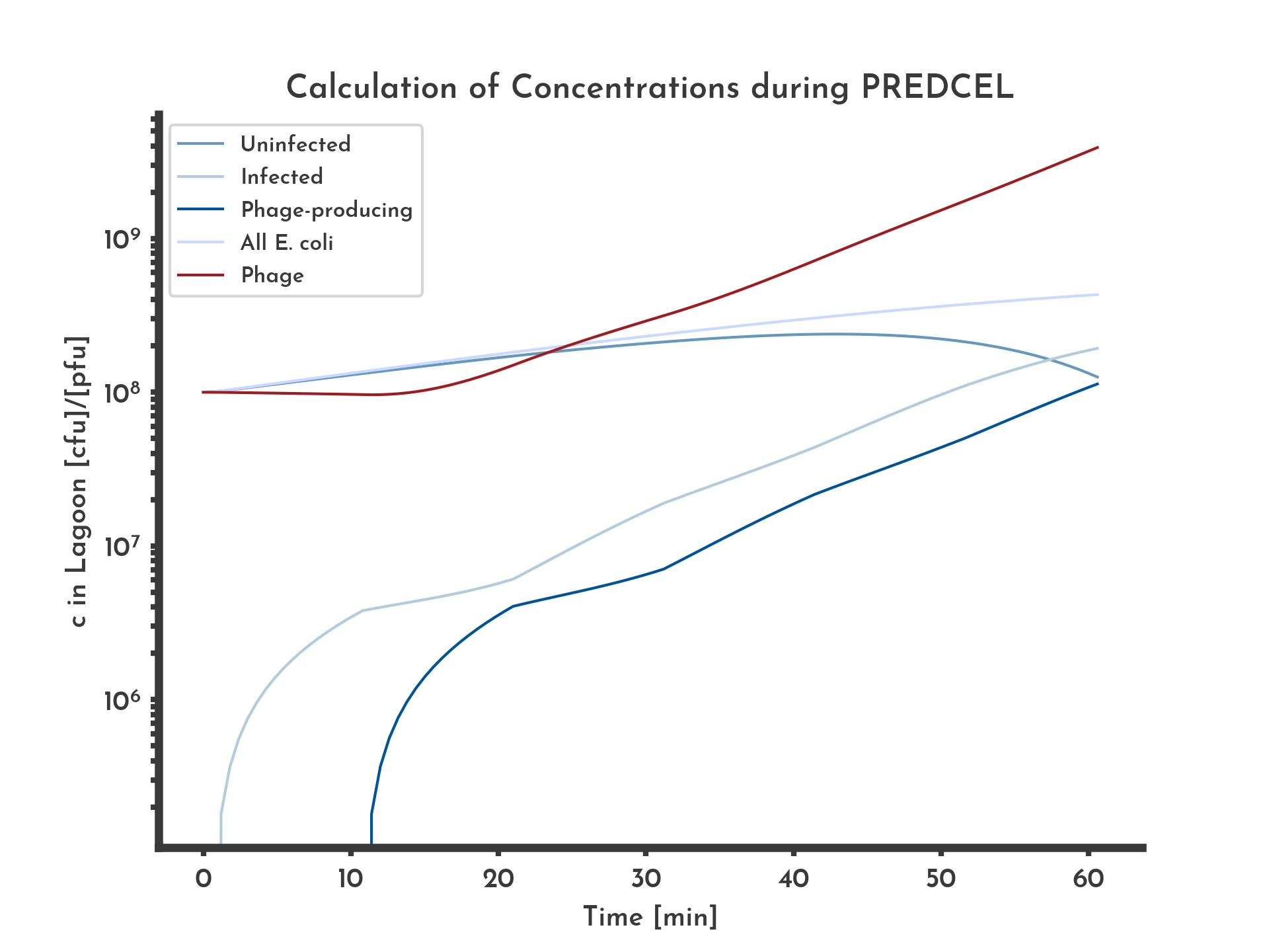
Figure 1: Basic logarithmic phage and E. coli titer plot with 20 % wildtype fitness
The blue lines correspond to the different E. coli populations. Exponential growth of E. coli and constant fitness of 20% of the wildtype, equal in all phages was assumed. After ten minutes infected E. coli start producing phage, corresponding to a stagnation in infected E. coli and an increase in phage concentration.
See the full list of parameters.
See the full list of parameters.
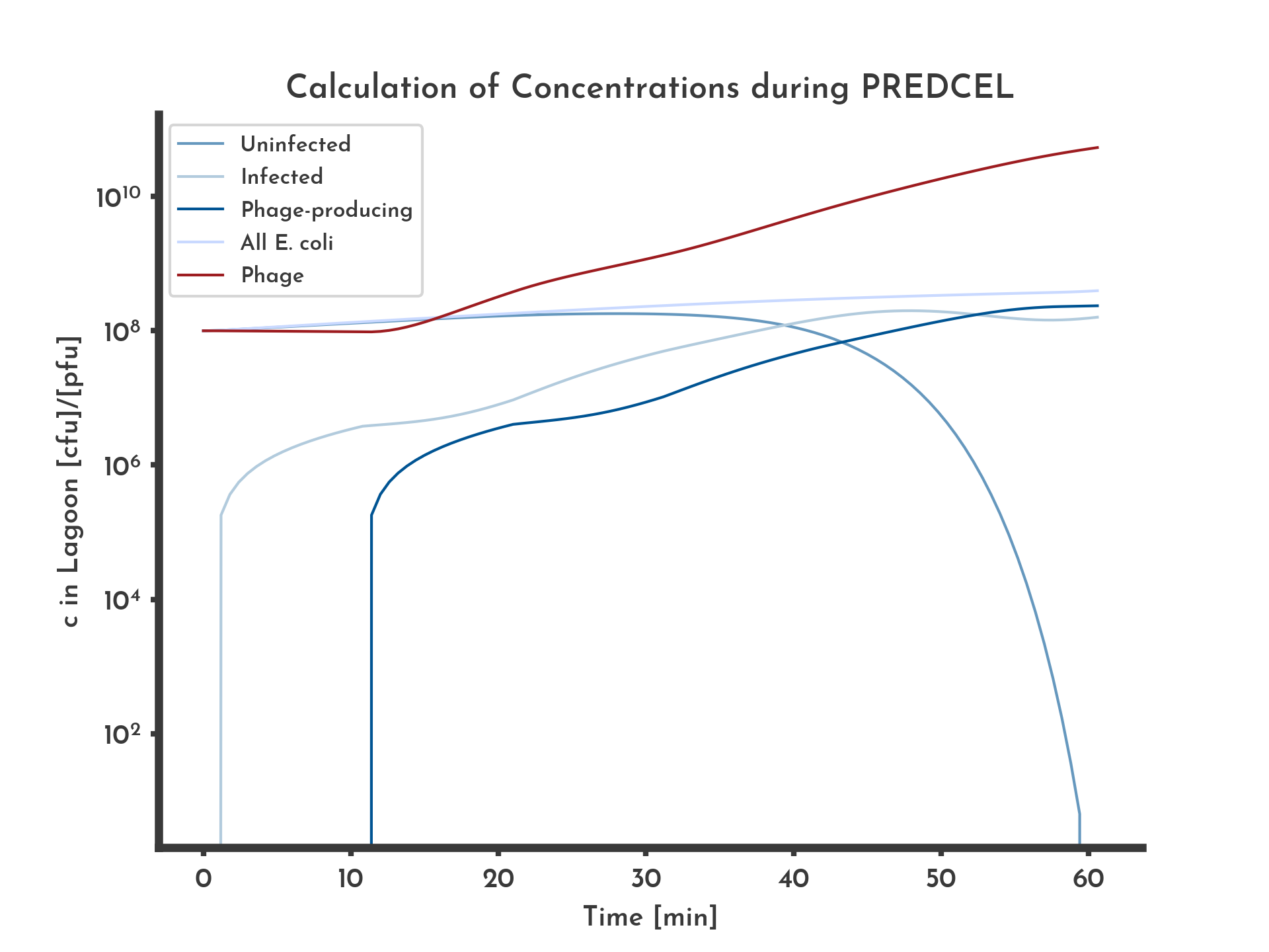
Figure 2: Basic logarithmic phage and E. coli titer plot with 100 % wildtype fitness.
The blue lines correspond to the different E. coli populations. Exponential growth of E. coli and constant fitness of 100% of the wildtype, equal in all phages was assumed. After ten minutes infected E. coli start producing phage, corresponding to a stagnation in infected E. coli and an increase in phage concentration.
See the full list of parameters.
See the full list of parameters.
Comparing the plots for 20 % (Fig. 1) and 100 % fitness (Fig. 2) show that a higher fitness increases the final phage titer and decreases the amount of uninfected E. coli earlier. The modeled concentrations include the concentration of uninfected, infected and phage-producing E. coli. They depend on each other as modeled below.
Modeling concentrations in one Lagoon
Here the concentrations \(c\) of uninfected E. coli, infected E. coli and phage producing E. coli as well as the M13 phage are modeled. They are denoted with the subscripts \(_{u}\), \(_{i}\), \(_{p}\) and \(_{P}\). If the whole E. coli population is referred to, \(c_{E}\) is used. If an arbitrary E. coli population is meant, the subscript \(_{e}\) is used. The phage concentration \(c_{P}\) refers to the free phage only, phage that are contained in an E. coli they infected are not included. The used parameters (Tab. 1) include the time \(t\), the affinity of phage for E. coli \(k\), the duration between infection of an E. coli and the first phage leaving the E. coli \(t_{P}\). The three different E. coli populations each have a generation time \(t\) that is denoted with their subscript. The fitness of a phage population is \(f\).Table 1: Variables and Parameters used in this model List of all paramters and variables used in this model. When possible values are given.
| Symbol | Name in source code | Value and Unit | Explanation |
|---|---|---|---|
| \(c \) | - | [cfu] or [pfu] | colony forming units for E. coli (cfu) or plaque forming units (pfu) for M13 phage |
| \( _u\) | - | - | Subscript for uninfected E. coli |
| \( _i\) | - | - | Subscript for infected E. coli |
| \( _p\) | - | - | Subscript for phage-producing E. coli |
| \( _e\) | - | - | Subscript any the of E. coli populations on its own |
| \( _E\) | - | - | Subscript for all populations of E. coli together |
| \( _P\) | - | - | Subscript for M13 phage |
| \(c_{c} \) | capacity |
[cfu/ml] | Maximum concentration of E. coli possible under given conditions, important for logistic growth |
| \(t\) | t |
[min] | Duration since the experiment modeled was started |
| \(t_{u} \) | tu |
\(20\) min | Duration one division of uninfected E. coli |
| \(t_{i} \) | ti |
\(30\) min | Duration one division of infected E. coli |
| \(t_{p} \) | tp |
\(40\) min | Duration one division of phage producing E. coli |
| \( t_{P}\) | tpp |
[min] | Duration between an E. coli being infected by an M13 phage and releasing the first new phage |
| \(g_{e} \) | e_growth_rate |
[cfu/min] | Growth rate of E. coli, depending on the type of growth (either logistic or exponential), the current concentration \(c_{e}\), the maximum concentration \(c_{c}\), and the generation time \(t_{e}\) |
| \( k\) | k |
\(3 \cdot 10^{-11}\frac{1}{cfu \cdot pfu \cdot ml \cdot min}\) | Affinity of M13 phage for E. coli |
| \( \mu_{max}\) | mumax |
\(16.67 \frac{cfu}{min \cdot ml \cdot cfu}\) | Wildtype M13 phage production rate |
| \( f\) | f |
? | Fitnessvalue, fraction of actual \(\mu\) and \(\mu_{max}\) |
Bacterial Growth
Each term describing the change of an E. coli concentration contains its growth, \(g_{e}\). The growth rate of an E. coli population can be modeled by exponential growth or by logistic growth. Especially, when long durations per lagoon are modeled, the logistic growth model is more realistic. In the exponential case the growth rate \(g_{e}\) is modeled as $$ g_{e} (t_{e}) = c_{e} \cdot \frac{log(2)}{t_{e} } $$ Note that the growth rate in the model increases over time, while in the modeled culture, the nutrient concentration decreases. That makes the logistic model more plausible, it models \(g_{e}\) as $$ g_{e} (t_{e}, \: c_{e}(t), \: c_{c}) = \frac{c_{c} - c_{e} (t)}{c_{c} } \cdot \frac{log(2)}{t_{e} } $$ In this case the growth rate decreases as the current concentration \(c_{e}\) approaches the maximum capacity for E. coli in the given setup \(c_{c}\). With this model \(c_{e} \leq c_{c}\) is true for any point in time.Transitions between uninfected, infected and phage-producing
Change of concentration of uninfected E. coli, \(\frac{\partial c_{u} }{\partial t} \: [cfu/min]\) $$ \frac{\partial c_{u} }{\partial t}(t) = g_{u} (t_{u}, \: c_{u}(t), \: c_{c}) - k \cdot c_{u}(t) \cdot c_{p}(t) $$ In addition to the growth term, the concentration of uninfected E. coli is described by a term for infection that takes into account the concentration of uninfected E. coli and the concentration of free phage and reduces the conentration of uninfected E. coli. The factor \(k\) is the affinity of phage for E. coli its value is \(k = 3 \cdot 10^{-11}\)Change of concentration of uninfected E. coli, \(\frac{\partial c_{i} }{\partial t} \: [cfu/min]\) $$ \frac{\partial c_{i} }{\partial t}(t) = \begin{cases} g_{i} (t_{i}, \: c_{i}(t), \:c_{c}) + k \cdot c_{i}(t) \cdot c_{p}(t) - c_{i}(t - t_{P}), \quad \text{for} \: t > t_{P} \\ g_{i} (t_{i}, \: c_{i}(t), \: c_{c}) + k \cdot c_{i}(t) \cdot c_{p}(t), \quad \text{otherwise} \end{cases} $$ Until \(t > t_{P}\) the concentration of infected E. coli increases by growth and infection of previouly uninfected E. coli. When \(t > t_{P}\), a third term describing that infected E. coli turn into phage-producing E. coli is subtracted. Change of concentration of phage producing E. coli, \(\frac{\partial c_{p} }{\partial t} \: [cfu/min]\) $$ \frac{\partial c_{p} }{\partial t}(t) = \begin{cases} g_{p} (t_{p}, \: c_{p}(t), \: c_{c}) - c_{i}(t - t_{P}), \quad \text{for} \: t > t_{P} \\ g_{p} (t_{p}, \: c_{p}(t), \: c_{c}), \quad \text{otherwise} \end{cases} $$ The population of phage producing E. coli only increases by growth until \(t > t_{P}\). When infected E. coli drop their first phage they turn into producing E. coli as described by the second term.
Phage propagation
Change of concentration of M13 phage, \(\frac{\partial c_{P} }{\partial t} \: [cpu/min]\) $$ \frac{\partial c_{P} }{\partial t}(t) = c_{P}(t) \cdot \mu_{max} \cdot f - k \cdot c_{u}(t)\cdot c_{P}(t) $$ The phage concentration is only increased by phage that leave phage-producing E. coli, which happens at a rate of \(f \cdot \mu_{max}\) per time unit, with f being the fitness, a value between 0 and 1, equal to the share of the wildtype M13 phages fitness and \(\mu_{max}\) being the wildtype phages production rate. We assume that the only negative influence on the free phage titer is phage infecting E. coli, which depends on both the phage titer \(c_{P}\) and the titer of uninfected E. coli, \(c_{i}\). When the fitness is assumed to be the same for all phages, it is modeled to be constant during the time in one lagoon (Fig. 3). A mode that implements an increase at each transfer is available.Numeric solutions
The problem described above is a system of four differential equations, of which two ( \(\frac{\partial c_{i} }{\partial t} \:, \: \frac{\partial c_{p} }{\partial t}\) ) are so called delayed differential equations. They contain a term that needs to be evaluated at a timepoint in the past \(t - t_{P}\). A python script was used to solve the problem numerically, using the explicit Euler method. The basic idea is that from a point in time with all values and all derivatives values given, the next point in time can be calculated by assuming a linear progress between the two points. $$ f(t_{n+1}) = f(t_{n}) + (t_{n+1} - t_{n}) \cdot f'(t_{n}) $$ This is performed for \(c_{u}(t)\), \(c_{i}(t)\), \(c_{p}(t)\) and \(c_{P}(t)\) rotatory, to always have the needed values from \(t_{n}\) ready for \(t_{n+1}\).The numeric solution of the model includes parameters like the number of steps \(s\) that are needed for the calculation but have no biological relevance, they are listed below (Tab. 1).
Table 2: Additional Variables and Parameters used in the numeric solution of the model List of all additional paramters and variables used in the numeric solution of this model. When possible values are given.
| Symbol | Name in Source code | Value and Unit | Explanation |
|---|---|---|---|
| \(v_{l}\) | vl |
[ml] | Volume of lagoon |
| \(t_{l} \) | tl |
[min] | Duration until transfer to the next lagoon |
| \(c_{u}(t_{0})\) | ceu0 |
[cfu] | Concentration of E. coli in a lagoon when M13 phages are transfered to it |
| \(c_{P}(t_{0})\) | cp0 |
[pfu] | Initial concentration of M13 phage in the first lagoon |
| \(n\) | epochs |
- | Number of epochs that are modeled, one epoch being everything that happens in one particular lagoon |
| \(s\) | tsteps |
- | Number of time steps for which numeric solutions are calculated, counted per epoch |
| \(c_{P}^{min}\) | min_cp |
[pfu] | Lower threshold for valid phage titers |
| \(c_{P}^{max}\) | max_cp |
[pfu] | Upper threshold for valid phage titers |
Fitness distributions
If a fitness distribution is assumed, the fitness does not necessarily stay constant in one lagoon. That means other than in the fitness models that as The distribution is initialized with 100 % of the phages having the starting fitness. First changes in the fitness distribution occur after the first E. coli start to release phages (Fig.4).The fitness distribution is modeled to change by mutation and selection. The selection is implemented in the following equation: $$ s_{i}(t_{n + 1}) = f_{i}(t_{n}) \cdot s_{i}(t_{n}) $$ \(f_{i}\) is one of \(N\) fitness values, \(s_{i}\) is the share of phages with that fitness value relative to the total phage population. Since the fitness is interpreted as a percentage of the wildtype fitness in this model, the new shares can be calculated als the product of the fitness value \(f_{i}\) and its old share \(s_{i}(t_{n})\). The resulting values are then normalized by divsion with $$ \sum_{i = 0}^{N} f_{i}(t_{n + 1}) $$ in order to always have shares that sum up to 1.
The mutation is implemented as a function that manipulates the fitness shares and applied to the fitness shares after selection. Here, \(r_{M}\) is the mutation rate, that means the amount of the fitness share \(i\) that changed during the mutation. \(w\) is the width of a fitness bin: $$ w = \frac{1}{N - 1} $$ The new shares are calculated as $$ s_{i}(t_{n + 1}) = \big(1 - r_{M}\big) \cdot s_{i}(t_{n}) + r_{M} \sum_{i = 0}^{N} \int_{f_{i} - \frac{1}{2} \cdot w}^{f_{i} + \frac{1}{2} \cdot w} \mathcal{N}_{\mu=f_{i}, \: \sigma}(x) \: dx $$ Special cases:
For \(f_{0}\) the integral is changed to $$ \int_{- \infty }^{f_{0} + \frac{1}{2} \cdot w} \mathcal{N}_{\mu=f_{i}, \: \sigma}(x) \: dx $$ For \(f_{0}\) the integral is changed to $$ \int_{f_{N} - \frac{1}{2} \cdot w}^{\infty} \mathcal{N}_{\mu=f_{i}, \: \sigma}(x) \: dx $$ to have the integrals over the normal distribution add up to 1. The normal distribution \(\mathcal{N}\) is used to model that many mutations have only small effects on the fitness, while some have a larger effect. \(\sigma\) is a parameter of the model that influences how much the new scores differ from the previous ones (Fig. 5). In this model it is theoretically possible that mutation turns any given fitness into any other fitness, however small values for can \(\sigma\) prevent this.
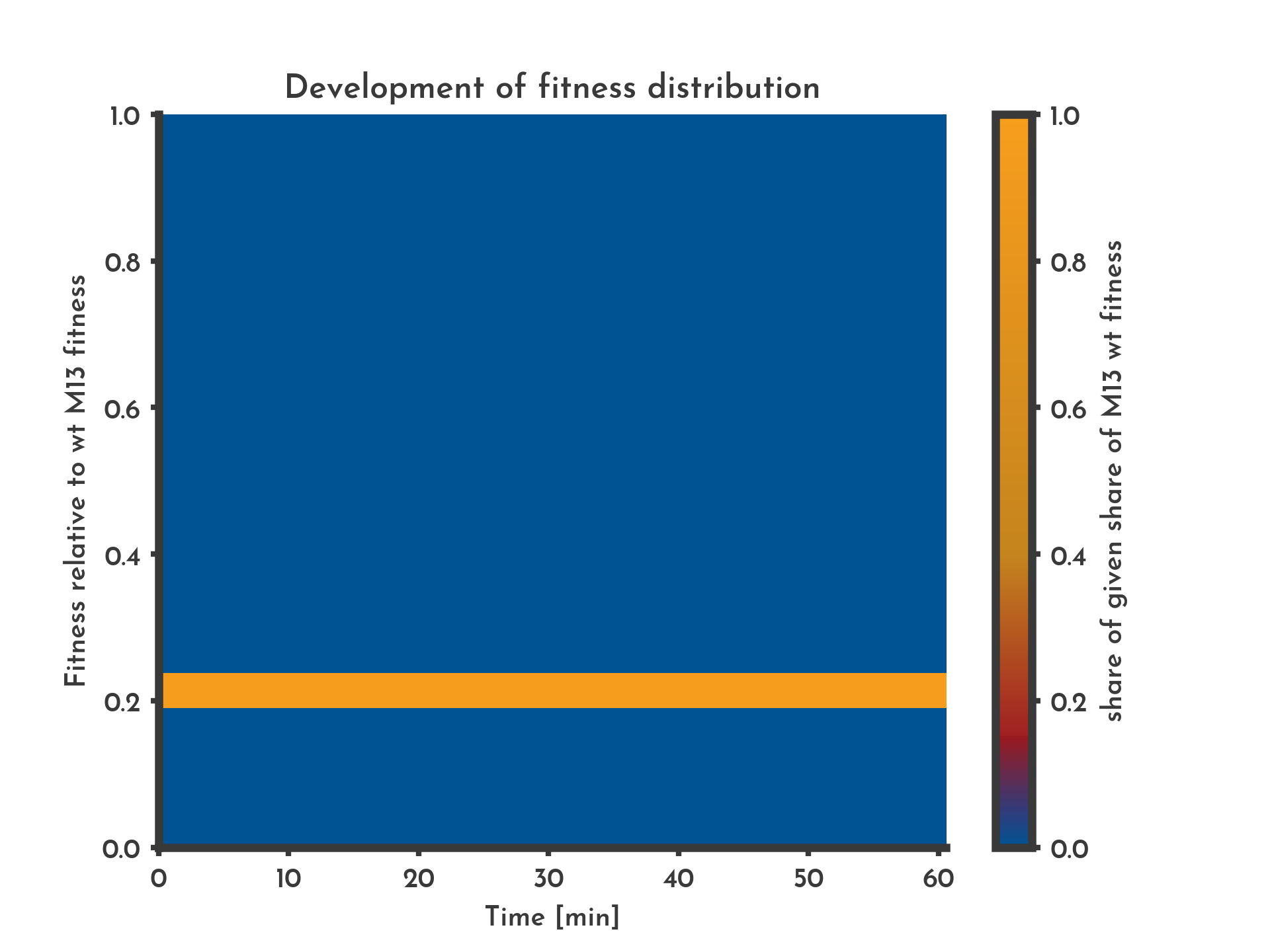
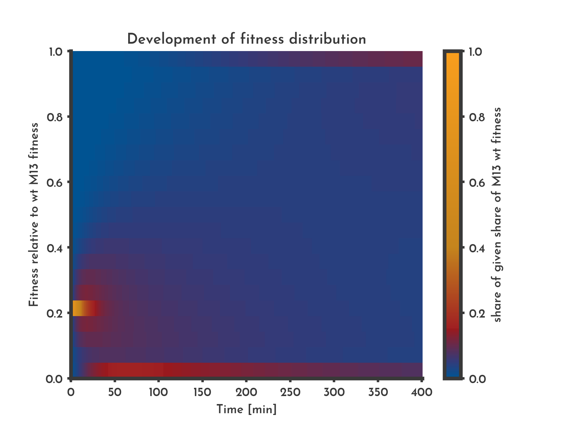
Figure 3: Constant fitness assumed to be equal for all phages in the lagoon
The color indicates the share of phages that have a specific fitness (y-axis) at a given time (x-axis). With the constant non-distributional mode the complete phage population has the initial fitness for the whole time.
See the full list of parameters.
See the full list of parameters.
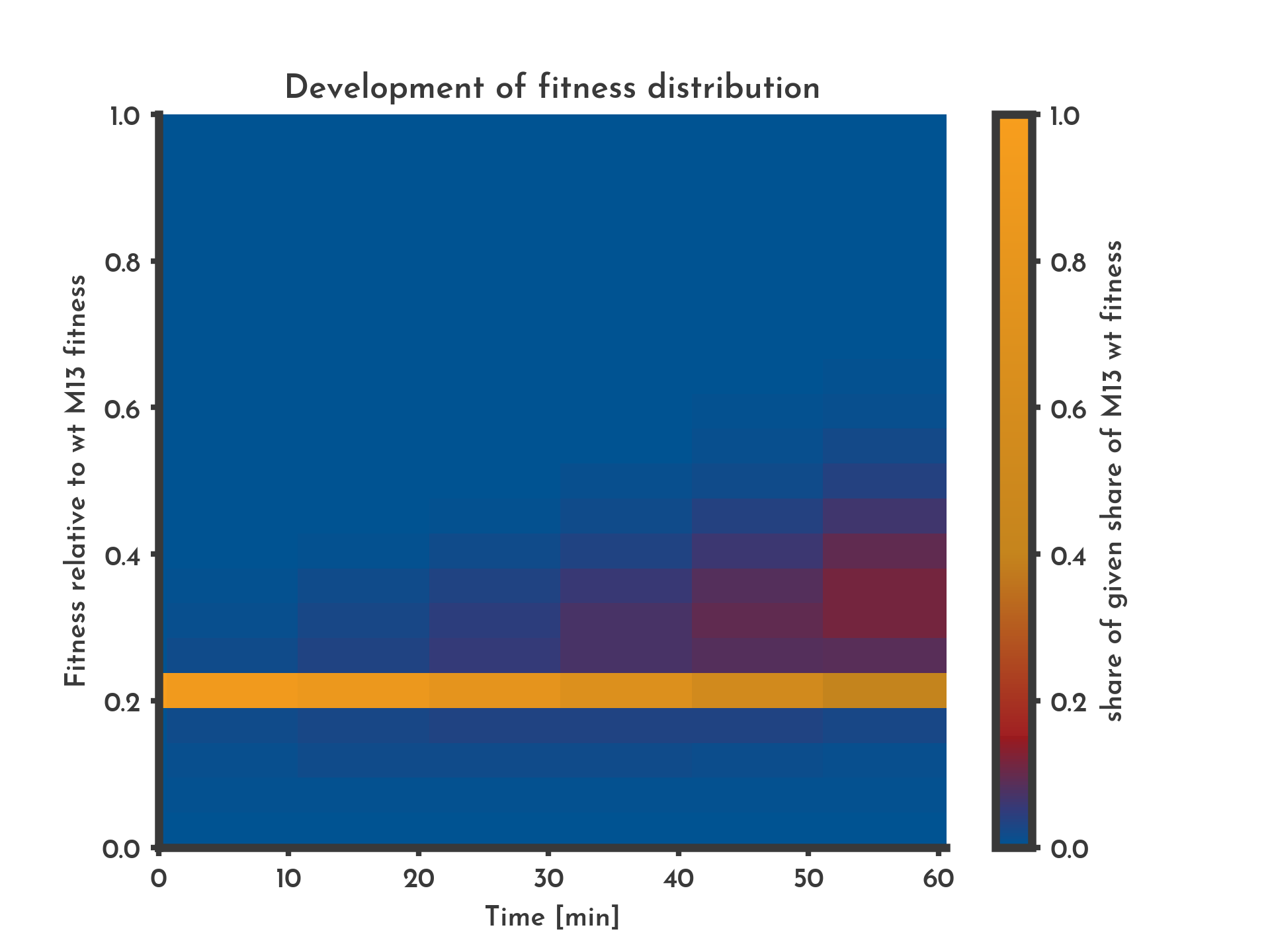
Figure 4: A distribution of fitness assumed with 10 % of new phages being subjected to changes in fitness.
The color indicates the share of phages that have a specific fitness (y-axis) at a given time (x-axis). With the distributional fitness mode after 10 minutes variants with a higher fitness occur.
See the full list of parameters.
See the full list of parameters.
When the the concentrations are modeled over a longer period of time the fitness of the wildtype is reached (Fig. 6). To more accurate model evolution in which the wildtype fitness is never reached, \(\mu_{max}\) can be set to a smaller value. This value will be reached by most of the phages, if enough time is given. Finally almost no phages with the lowest fitness can be found in the lagoon (Fig. 7).
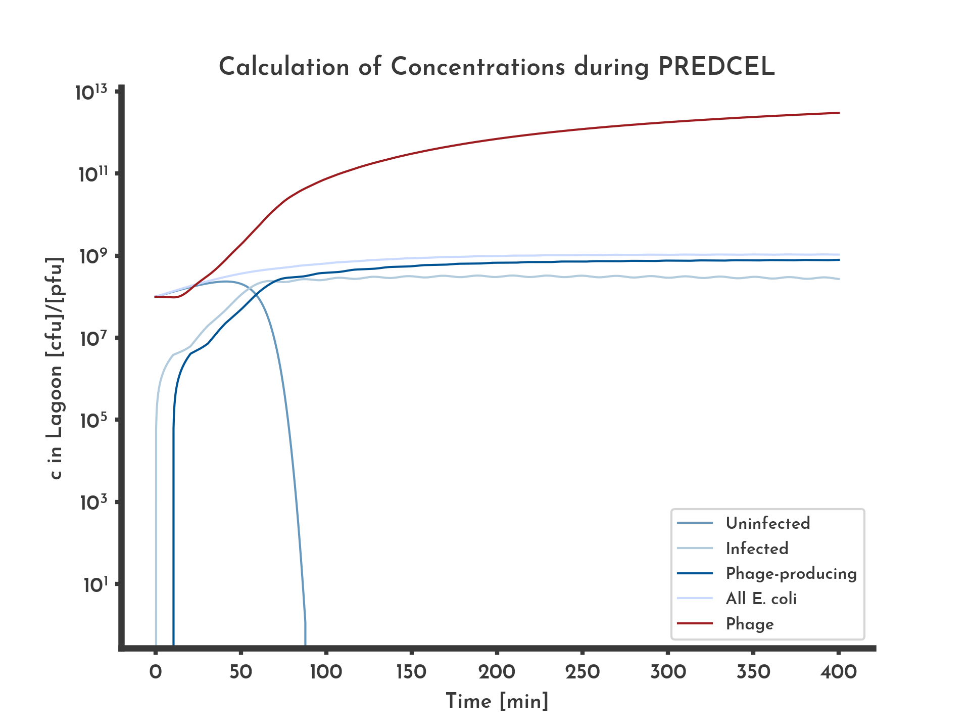
Figure 5: E. coli and phage titer modled over 6.5 h with a normal distribution based fitness distribution.
Blue lines correspond to E. coli titers, the red line is the total phage titer.
See the full list of parameters.
See the full list of parameters.
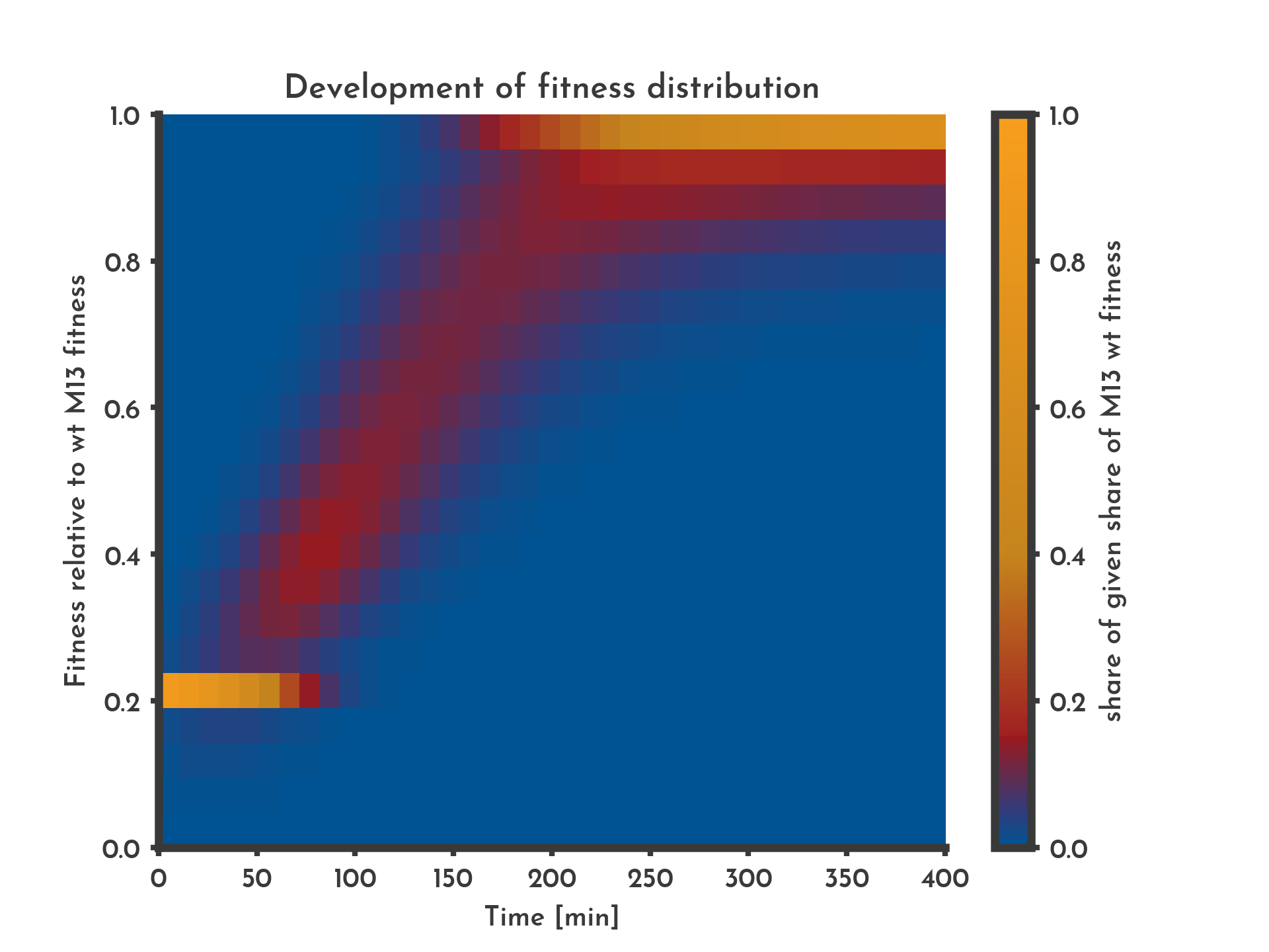
Figure 6: A distribution of fitness is assumed with 10 % of new phages being subjected to changes in fitness over 6.5 h.
The color indicates the share of phages that have a specific fitness (y-axis) at a given time (x-axis). After 4 h the system goes in a steay state where mutation and selection cancel each other out.
See the full list of parameters.
See the full list of parameters.
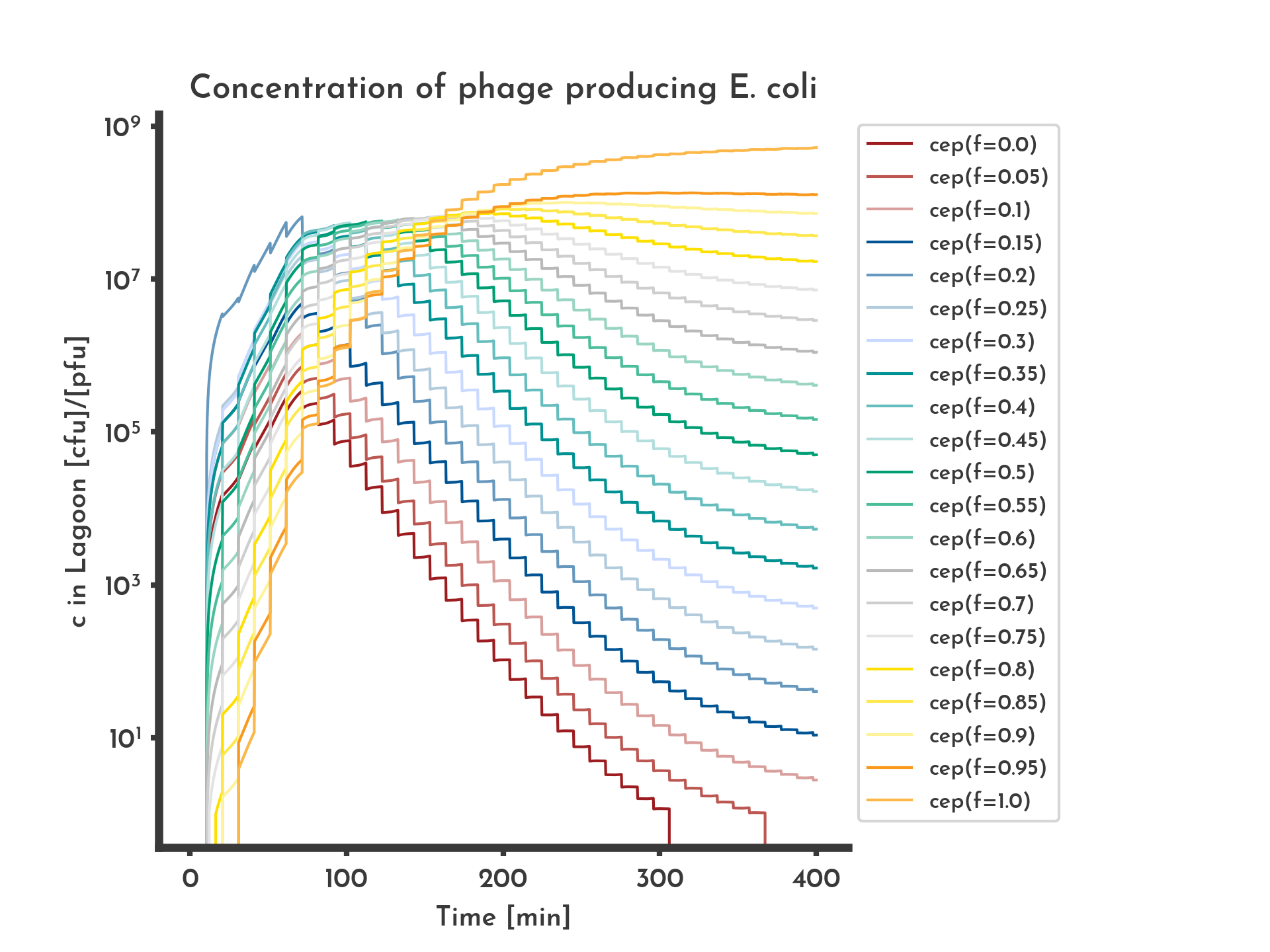
Figure 7: Shares of the phage-producing E. coli producing phages with different fitness values.
Modelled with normal distribution based mutation. 'cep(f=x)' denotes the concentration of phage-producing E. coli that produce phage with fitness x. Initially all phage-producing E. coli produce phage with 20 % of the wildtype fitness, they make up the largest share for 1 h after which fitter phage-producing E. coli take over the lagoon.
See the full list of parameters.
See the full list of parameters.
Since most mutations decrease fitness in reality, a symmetric function like the normal distributions density function may not be the best choice. Consequently we also implemented a mutation function with a skew normal distribution \(\mathcal{S}\), that replaces \(\mathcal{N}\). It has an additional parameter \(\alpha\) that modulates the skewness.
$$
s_{i}(t_{n + 1}) = \big(1 - r_{M}\big) \cdot s_{i}(t_{n}) + r_{M} \sum_{i = 0}^{N} \int_{f_{i} - \frac{1}{2} \cdot w}^{f_{i} + \frac{1}{2} \cdot w} \mathcal{S}_{\mu=f_{i}, \: \sigma, \: \alpha}(x) \: dx
$$
Special cases:
For \(f_{0}\) the integral is changed to $$ \int_{- \infty }^{f_{0} + \frac{1}{2} \cdot w} \mathcal{S}_{\mu=f_{i}, \: \sigma, \: \alpha}(x) \: dx $$ For \(f_{0}\) the integral is changed to $$ \int_{f_{N} - \frac{1}{2} \cdot w}^{\infty} \mathcal{S}_{\mu=f_{i}, \: \sigma, \: \alpha}(x) \: dx $$ to have the integrals over the normal distribution add up to 1.
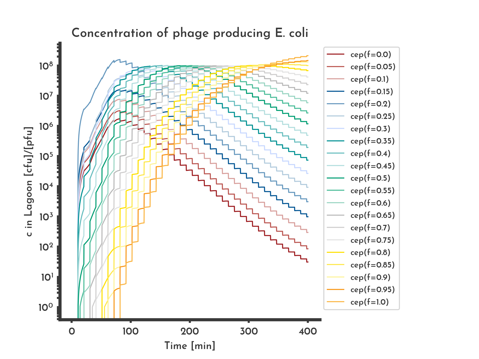
The equation for \(\frac{\partial c_{P} (t)}{\partial t}\) is changed into the following to incorporate the distributed fitness. $$ \frac{\partial c_{P} (t)}{\partial t} = -k \cdot c_{u}(t) \cdot c_{P} (t) + \sum_{i = 0}^N f_{i} \cdot s_{i} \cdot \mu \cdot c_{p} (t) $$ Using the skew normal distribution, the increase in fitness occurs later and lower fitness values occur for a longer period of time, since it takes longer for the higher fitness values to occur (Fig. 8).
For \(f_{0}\) the integral is changed to $$ \int_{- \infty }^{f_{0} + \frac{1}{2} \cdot w} \mathcal{S}_{\mu=f_{i}, \: \sigma, \: \alpha}(x) \: dx $$ For \(f_{0}\) the integral is changed to $$ \int_{f_{N} - \frac{1}{2} \cdot w}^{\infty} \mathcal{S}_{\mu=f_{i}, \: \sigma, \: \alpha}(x) \: dx $$ to have the integrals over the normal distribution add up to 1.
The equation for \(\frac{\partial c_{P} (t)}{\partial t}\) is changed into the following to incorporate the distributed fitness. $$ \frac{\partial c_{P} (t)}{\partial t} = -k \cdot c_{u}(t) \cdot c_{P} (t) + \sum_{i = 0}^N f_{i} \cdot s_{i} \cdot \mu \cdot c_{p} (t) $$ Using the skew normal distribution, the increase in fitness occurs later and lower fitness values occur for a longer period of time, since it takes longer for the higher fitness values to occur (Fig. 8).
Figure 8: Shares of the phage-producing E. coli producing phages with different fitness values.
Modeled with skew normal distribution based mutation biased towards lower fitness scores. Initially all phage-producing E. coli produce phage with 20 % of the wildtype fitness, they make up the largest share for 1 h after which fitter phage-producing E. coli take over the lagoon.
See the full list of parameters.
See the full list of parameters.
Other assumptions for the mutation function are possible, for example a function that randomly samples from a normal distribution but is biased towards mutations that decrease fitness.
Since this model of fitness and mutation is heavily abstracted the fitness distribution is most likely limeted to qualitative statements. Still it provides an intuitive understanding on how directed evolution can work and illustrates the role of selection and mutation. If the model without mutation (Fig. 3) is compared to one with mutation and selection (Fig. 6) role of mutation, diversificating the pool of phages can be seen. When comparing a model without selection (Fig. 9) to the one with mutation and selection (Fig. 6) the role of selection can be described as channeling the variants caused by mutation into a specific direction.
Since this model of fitness and mutation is heavily abstracted the fitness distribution is most likely limeted to qualitative statements. Still it provides an intuitive understanding on how directed evolution can work and illustrates the role of selection and mutation. If the model without mutation (Fig. 3) is compared to one with mutation and selection (Fig. 6) role of mutation, diversificating the pool of phages can be seen. When comparing a model without selection (Fig. 9) to the one with mutation and selection (Fig. 6) the role of selection can be described as channeling the variants caused by mutation into a specific direction.
Figure 9: Effect of missing selection
Without selection fitness does not show a clear trend until the boundary values show higher shares. This is most likely due to the equation that gives the boundary values fitness that leaves the interval [0, 1]. The color indicates the share of phages that have a specific fitness (y-axis) at a given time (x-axis).
See the full list of parameters.
See the full list of parameters.
Effects of noise
Errors in the parameters of the model can be due discrepancies of the modeled experiments conditions and the conditions under which parameters were determined. To make general statements on how sensitive the model reacts to noise in its parameters, a function was introduced that adds adjustable gaussian noise to all parameters. It was scaled relative to each parameters value. The function \(n(v)\) returns the noisy value of \(v\), the random argument \(r\) is sampled from a uniform distribution over \([0, 1]\). $$ n(v) = v + \big(1 - 2r\big) \cdot \sigma_{G} \cdot \sigma_{v} \cdot v, \quad r \in [0, 1] $$ \(\sigma_{G}\) is a global factor that is the same for all \(v\), \(\sigma_{v}\) is specific for \(v\). This makes it possible to have one parameter being noisier than another, while being able to tune the noise globally.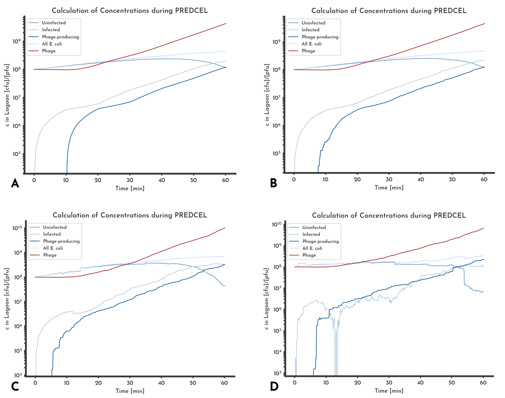
Figure 10: Comparison of different noise levels effects on predicted phage and E. coli titer.
Gaussian noise was added to all parameters relative to each parameter with a sigma of A: 0 %, B: 20 %, C: 50 %, D: 100 %. The overall behavior of the different titers stays the is the same, even when gaussian noise with a sigma of 100 % of the value is introduced. The strongest discrepancy between the noise free version (A) and the noisiest (B) is that the titer of uninfectd E. coli decreases below 1e3 multiple times.
See the full list of parameters.
See the full list of parameters.
The model seems to be sufficiently robust against random errors. However systematic errors in the parameters can still have a large effect on predicted phage and E. coli titers.
Modeling concentrations over multiple Lagoons
PREDCEL is based on transferring phage from one lagoon into the next. This substitutes the constant supply with fresh medium, fresh E. coli and the constant dilution by a turbidostat. Because transferring decreases the phage by the relation of the transfer volume \(V_{t}\) to the lagoon volume \(v_{L}\), there is an increased risk of washout. This model is partly motivated by the goal to minimize that risk (Fig. 11). The basic idea is to enable the user to react to a diminishig phage titer early enough while maintaining a reasonable level of monitoring.In all following model versions, a distributional fitness, transfer of phage and E. coli and logistic growth are assumed. Due to their lower plausibility the alternatives are not shown, but are available as functions in the script.
When transfer from one volume to the next is performed, the new lagoon can be modeled with starting values calculated from the last lagoons end values. For each concentration from the previous lagoon \(c_{t}\), the concentration in the next lagoon \(c_{t+1}\) is calculated as $$ c_{t+1} = \frac{v_{t} }{v_{l} } \cdot c_{t} $$ with \(v_{L}\), the volume of a lagoon and \(v_{t}\), the volume that is transferred.
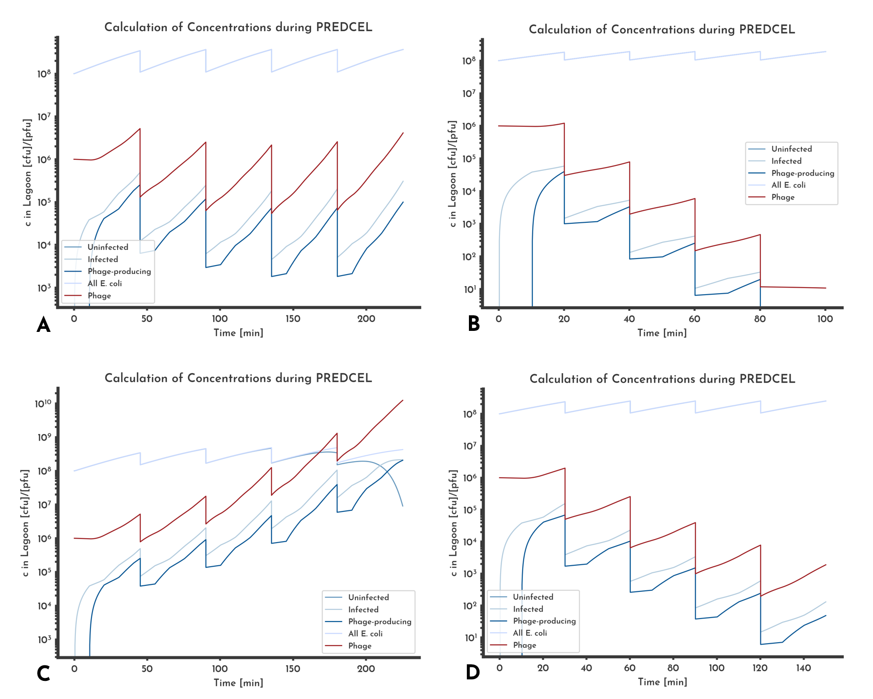
Figure 11: Different phage titer trends
In A the phage titer just before the transfer is constant, that corresponds with a constant MOI that can be set by choosing the initial phage titer. In B washout occurs, after the fifth transfer no phage will be left. C shows an increase in phage titer, D a decrease
See the full list of parameters.
See the full list of parameters.
If the transfered volume is spinned down before it is added to the new lagoon, the initial value for \(c_{P}\) is calculated this way. The initial concentration of uninfected E. coli is set to the initial cell density. Initial concentrations of infected and phage-producing E. coli are set to zero, because before the transfer, no phages are present in the new lagoon.
If the transfer volume is not spinned down, the concentration of infected and phage-producing E. coli are calculated, using the above formula. The initial concentration of uninfected E. coli is the calculated the same way, but the initial cell density is added.
The differences are shown in Figure 12.

Figure 12: Effect of transferring phage only
Plots A and C are from the same model, as well as B and D. 'cep(f=x)' denotes the concentration of phage-producing E. coli that produce phage with fitness x. When only phage is transferred, the phage-producing E. coli population has to be rebuilt after each transfer, seen as the decreases to zero in A. If only phage is transferred, variants with a low fitness score are washed out earlier than if the phage-producing E. coli are transferred too.
See the full list of parameters.
See the full list of parameters.
Comparison to data from CYP1A2-PREDCEL
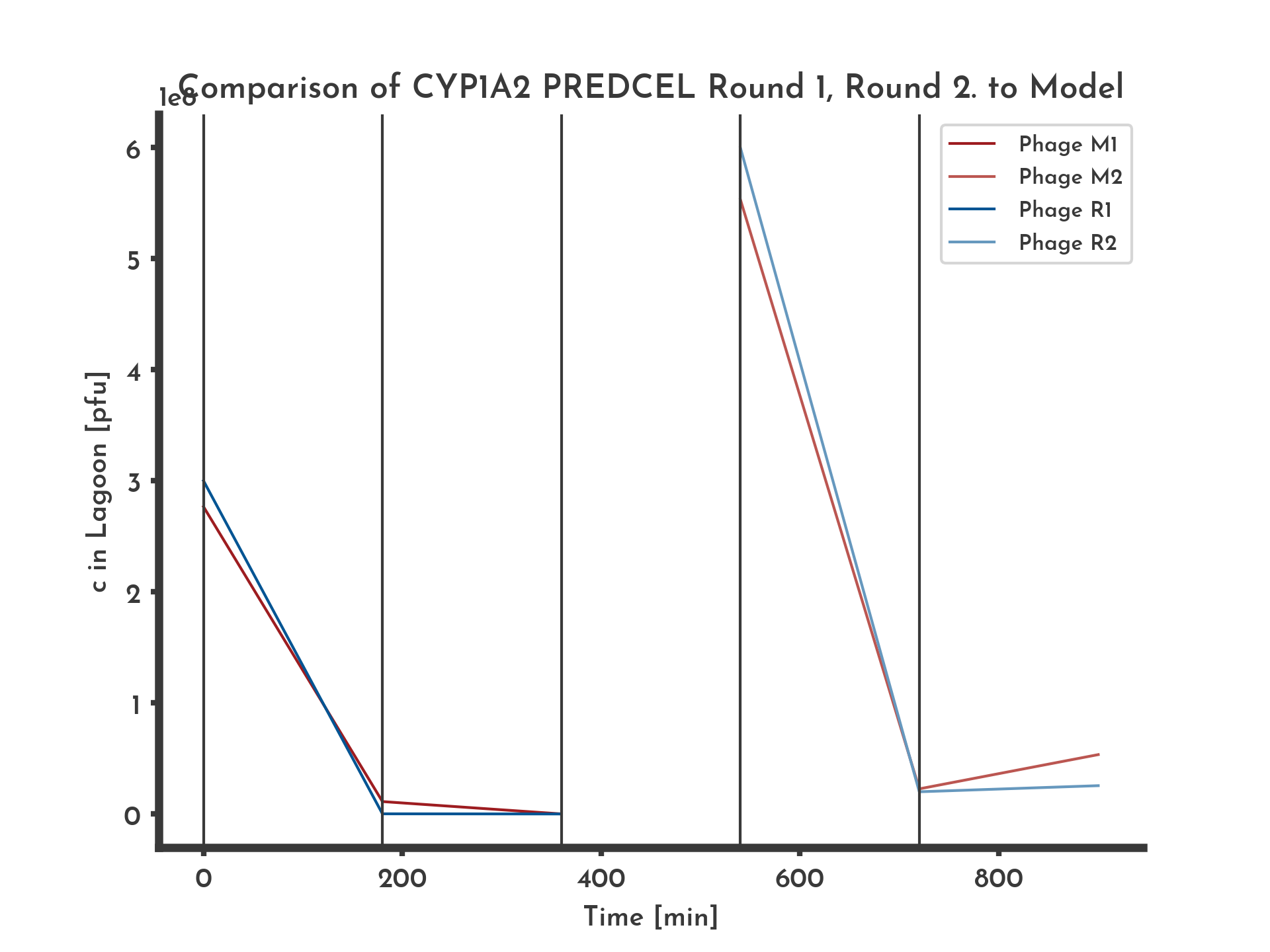
Figure 13: Phage titer modeled in two setups compared to two rounds of CYP1A2-PREDCEL
The two rounds of PREDCEL each consisted of one transfer, in between the phage was amplificated without selection pressure on the CYP1A2. The model was only adjusted in the assumed fitness in between the two rounds of PREDCEL.
See the full list of parameters.
See the full list of parameters.
To asses the model in comparison with real data, phage titers from CYP1A2-PREDCEL were modeled with different values for the unkown parameters and the set of parameters that described the data best was chosen (Fig. 13).
The phage titer data consists of two sets, a first round of PREDCEL with 1 transfer, followed by amplification of the resulting library on a strain that allows the phage to propagate independent of the performance of their CYP1A2 sequence. Then a second round of PREDCEL with one transfer was done. The time between two transfers \(t_{L}\) was 3 h, the lagoon volume \(v_{L}\) 20 ml and the transferred volume \(v_{T}\) 3 ml. Unknown parameters are the initial fitness, how the fitness changes and the phage degradation rate \(r_{D}\).
Both round were best described an initial fitness of \(f(t_{0}) = 0.001\), and a degration rate of \(r_{D} = 0.075\). For the first round constant fitness was assumed, since the initial library complexity is 1 and a sufficiently sized library is a maijor requirement for fitness to rise. For the second round the starting fitness was assumed to be identical to the fitness of the first round, then increasing to \(f(t_{0}) = 0.025\) after the transfer.
The initial phage titers for both rounds were given in the data. The full conditions for both models and the full data is available below.
Finding Parameters
Combinations of parameters that result in maintaing an acceptable phage titer most easily be found by calculating the phage titers for different sets parameters systematically. For this purpose a function was implemented that systematically tries all combinations of a given number \(n\) different values for the initial fitness \(f_{0}\), the time in one lagoon \(t_{L}\) and the transferred volume \(v_{t}\). A tunable parameter \(\delta\) defines how the range over wich the \(n\) values for one of the parameters are spread relative to the value of the parameter. For each parameter \(p\) the tried values are in $$ \Big\{p + \big(1 - \delta \big) + i \frac{2 \delta}{n - 1} \cdot p \: \Big\vert \: i = 0, ..., (n - 1)\Big\} $$
In directed evolution the fitness should increase over time. A linear increase in fitness between to given values was implemented to show this. The problem with this approach is its basic assumption being that all phage-producing E. coli are infected by phages with the same fitness.
To make the model more plausible, a distribution of fitness was introduced. For a set of discrete fitness values each fitness values share of the phage-producing E. coli population is calculated.
That changes the equation for the change in the concentration of phage-producing E. coli to
The calculation is for \(N\) different fitness values \(f_{i}\) and their share of the total phage-producing E. coli population \(s_{i}\).
Figure 14: Tendency of Phage titer modeled in 8000 setups - Fitness variable
The phage titer was modelled for 8000 setups with 20 values each for \(f_{0}\), \(\frac{v_{t} }(v_{L}\) and \(t_{L}\), in a range of \(\pm 75 \) % of the original value. The color indicates the tendency of the phage titer just before the transfer: Blue indicates a decrease, red a constant phage titer and yellow an increase. The values were obtained by setting an upper and a lower threshold for the phage titer and counting the number of transfers in which the phage titer stayed within these.
See the full list of parameters.
See the full list of parameters.
Figure 15: Tendency of Phage titer modeled in 8000 setups - Transfer Volume variable
The phage titer was modelled for 8000 setups with 20 values each for \(f_{0}\), \(\frac{v_{t} }(v_{L}\) and \(t_{L}\), in a range of \(\pm 75 \) % of the original value. The color indicates the tendency of the phage titer just before the transfer: Blue indicates a decrease, red a constant phage titer and yellow an increase. The values were obtained by setting an upper and a lower threshold for the phage titer and counting the number of transfers in which the phage titer stayed within these.
See the full list of parameters.
See the full list of parameters.
Figure 16: Tendency of Phage titer modeled in 8000 setups - Time until transfer variable
The phage titer was modelled for 8000 setups with 20 values each for \(f_{0}\), \(\frac{v_{t} }(v_{L}\) and \(t_{L}\), in a range of \(\pm 75 \) % of the original value. The color indicates the tendency of the phage titer just before the transfer: Blue indicates a decrease, red a constant phage titer and yellow an increase. The values were obtained by setting an upper and a lower threshold for the phage titer and counting the number of transfers in which the phage titer stayed within these.
See the full list of parameters.
See the full list of parameters.
When phages have a high fitnes, and both the ratio of transfer volume to lagoon volume and the time in lagoon have high values too, the phage titer increases over time (Fig. 14 - 16). If however all three values are low, the risk of washout rises.
Parameters used for the figures
Figure 1, 3 - 20 % fitness
 'capacity': 1000000000.0,
 'ceu0': 100000000.0,
 'cp0': 100000000.0,
 'epochs': 1,
 'f0': 0.2,
 'f_prec': 21,
 'fend': 1.0,
 'fitnessmode': 'dist',
 'ftype': 'const',
 'growth_mode': 'logistic',
 'k': 3e-11,
 'max_cp': 2000000000.0,
 'min_cp': 100000.0,
 'mumax': 16.667,
 'mutation_dist': 'norm',
 'noisy': 0.0,
 'phageonly': 'True',
 'plot_dist': 'True',
 'sigma': 0.0,
 'skewness': 1.0,
 'ti': 30,
 'tl': 60,
 'to_mutate': 0.0,
 'tp': 40,
 'tpp': 10,
 'tsteps': 100,
 'tu': 20,
 'vl': 20,
 'vt': 1
Figure 2 - 100 % fitness
 'capacity': 1000000000.0,
 'ceu0': 100000000.0,
 'cp0': 100000000.0,
 'epochs': 1,
 'f0': 1.0,
 'f_prec': 21,
 'fend': 1.0,
 'fitnessmode': 'const',
 'ftype': 'const',
 'growth_mode': 'logistic',
 'k': 3e-11,
 'max_cp': 2000000000.0,
 'min_cp': 100000.0,
 'mumax': 16.667,
 'mutation_dist': 'norm',
 'noisy': 0.0,
 'phageonly': 'True',
 'plot_dist': 'False',
 'sigma': 0.001,
 'skewness': 1.0,
 'ti': 30,
 'tl': 60,
 'to_mutate': 0.0,
 'tp': 40,
 'tpp': 10,
 'tsteps': 100,
 'tu': 20,
 'vl': 20,
 'vt': 1
Figure 4 - Distributional fitness 1 h
 'capacity': 1000000000.0,
 'ceu0': 100000000.0,
 'cp0': 100000000.0,
 'epochs': 1,
 'f0': 0.2,
 'f_prec': 21,
 'fend': 1.0,
 'fitnessmode': 'dist',
 'ftype': 'const',
 'growth_mode': 'logistic',
 'k': 3e-11,
 'max_cp': 2000000000.0,
 'min_cp': 100000.0,
 'mumax': 16.667,
 'mutation_dist': 'norm',
 'noisy': 0.0,
 'phageonly': 'True',
 'plot_dist': 'True',
 'sigma': 0.0,
 'skewness': 1.0,
 'ti': 30,
 'tl': 60,
 'to_mutate': 0.0,
 'tp': 40,
 'tpp': 10,
 'tsteps': 100,
 'tu': 20,
 'vl': 20,
 'vt': 1
Figure 5, 6, 7 - Distributional fitness 6.5 h
 'capacity': 1000000000.0,
 'ceu0': 100000000.0,
 'cp0': 100000000.0,
 'epochs': 1,
 'f0': 0.2,
 'f_prec': 21,
 'fend': 1.0,
 'fitnessmode': 'dist',
 'ftype': 'const',
 'growth_mode': 'logistic',
 'k': 3e-11,
 'max_cp': 2000000000.0,
 'min_cp': 100000.0,
 'mumax': 16.667,
 'mutation_dist': 'norm',
 'noisy': 0.0,
 'phageonly': 'True',
 'plot_dist': 'True',
 'sigma': 0.1,
 'skewness': 1.0,
 'ti': 30,
 'tl': 400,
 'to_mutate': 0.1,
 'tp': 40,
 'tpp': 10,
 'tsteps': 2000,
 'tu': 20,
 'vl': 20,
 'vt': 1
Figure 8 - Distributional fitness skew
 'capacity': 1000000000.0,
 'ceu0': 100000000.0,
 'cp0': 100000000.0,
 'epochs': 1,
 'f0': 0.2,
 'f_prec': 21,
 'fend': 1.0,
 'fitnessmode': 'dist',
 'ftype': 'const',
 'growth_mode': 'logistic',
 'k': 3e-11,
 'max_cp': 2000000000.0,
 'min_cp': 100000.0,
 'mumax': 16.667,
 'mutation_dist': 'skew',
 'noisy': 0.0,
 'phageonly': 'True',
 'plot_dist': 'True',
 'sigma': 0.1,
 'skewness': -1.0,
 'ti': 30,
 'tl': 400,
 'to_mutate': 0.1,
 'tp': 40,
 'tpp': 10,
 'tsteps': 2000,
 'tu': 20,
 'vl': 20,
 'vt': 1
Figure 9 - Distributional fitness without selection
 'capacity': 1000000000.0,
 'ceu0': 100000000.0,
 'cp0': 100000000.0,
 'epochs': 1,
 'f0': 0.2,
 'f_prec': 21,
 'fend': 1.0,
 'fitnessmode': 'dist',
 'ftype': 'const',
 'growth_mode': 'logistic',
 'k': 3e-11,
 'max_cp': 2000000000.0,
 'min_cp': 100000.0,
 'mumax': 16.667,
 'mutation_dist': 'norm',
 'noisy': 0.0,
 'phageonly': 'True',
 'plot_dist': 'True',
 'sigma': 0.1,
 'skewness': -1.0,
 'ti': 30,
 'tl': 400,
 'to_mutate': 0.1,
 'tp': 40,
 'tpp': 10,
 'tsteps': 500,
 'tu': 20,
 'vl': 20,
 'vt': 1
Figure 10 - Effects of different noise levels
 'capacity': 1000000000.0,
 'ceu0': 100000000.0,
 'cp0': 100000000.0,
 'epochs': 1,
 'f0': 0.2,
 'f_prec': 21,
 'fend': 1.0,
 'fitnessmode': 'dist',
 'ftype': 'const',
 'growth_mode': 'logistic',
 'k': 3e-11,
 'max_cp': 2000000000.0,
 'min_cp': 100000.0,
 'mumax': 16.667,
 'mutation_dist': 'skew',
 'noisy': 0.05,  # or 0.1, 0.2, 0.5
 'phageonly': 'True',
 'plot_dist': 'True',
 'sigma': 0.1,
 'skewness': -1.0,
 'ti': 30,
 'tl': 60,
 'to_mutate': 0.1,
 'tp': 40,
 'tpp': 10,
 'tsteps': 500,
 'tu': 20,
 'vl': 20,
 'vt': 1
Figure 11A - Constant Phage Titer
 'capacity': 1000000000.0,
 'ceu0': 100000000.0,
 'cp0': 1000000.0,
 'epochs': 5,
 'f0': 0.1,
 'f_prec': 11,
 'fend': 1.0,
 'fitnessmode': 'dist',
 'ftype': 'const',
 'growth_mode': 'logistic',
 'k': 3e-11,
 'max_cp': 2000000000.0,
 'min_cp': 100000.0,
 'mumax': 16.667,
 'mutation_dist': 'norm',
 'noisy': 0.0,
 'phageonly': 'False',
 'plot_dist': 'True',
 'sigma': 0.025,
 'skewness': -1.0,
 'ti': 30,
 'tl': 45,
 'to_mutate': 0.025,
 'tp': 40,
 'tpp': 10,
 'tsteps': 200,
 'tu': 20,
 'vl': 20,
 'vt': 0.5
Figure 11B - Washout
 'capacity': 1000000000.0,
 'ceu0': 100000000.0,
 'cp0': 1000000.0,
 'epochs': 5,
 'f0': 0.1,
 'f_prec': 11,
 'fend': 1.0,
 'fitnessmode': 'dist',
 'ftype': 'const',
 'growth_mode': 'logistic',
 'k': 3e-11,
 'max_cp': 2000000000.0,
 'min_cp': 100000.0,
 'mumax': 16.667,
 'mutation_dist': 'norm',
 'noisy': 0.0,
 'phageonly': 'False',
 'plot_dist': 'True',
 'sigma': 0.025,
 'skewness': -1.0,
 'ti': 30,
 'tl': 20,
 'to_mutate': 0.025,
 'tp': 40,
 'tpp': 10,
 'tsteps': 200,
 'tu': 20,
 'vl': 20,
 'vt': 0.5
Figure 11C - Increase in Phage Titer
 'capacity': 1000000000.0,
 'ceu0': 100000000.0,
 'cp0': 1000000.0,
 'epochs': 5,
 'f0': 0.1,
 'f_prec': 11,
 'fend': 1.0,
 'fitnessmode': 'dist',
 'ftype': 'const',
 'growth_mode': 'logistic',
 'k': 3e-11,
 'max_cp': 2000000000.0,
 'min_cp': 100000.0,
 'mumax': 16.667,
 'mutation_dist': 'norm',
 'noisy': 0.0,
 'phageonly': 'False',
 'plot_dist': 'True',
 'sigma': 0.025,
 'skewness': -1.0,
 'ti': 30,
 'tl': 45,
 'to_mutate': 0.025,
 'tp': 40,
 'tpp': 10,
 'tsteps': 200,
 'tu': 20,
 'vl': 20,
 'vt': 3
Figure 11D - Decrease in Phage Titer
 'capacity': 1000000000.0,
 'ceu0': 100000000.0,
 'cp0': 100000000.0,
 'epochs': 1,
 'f0': 0.2,
 'f_prec': 21,
 'fend': 1.0,
 'fitnessmode': 'dist',
 'ftype': 'const',
 'growth_mode': 'logistic',
 'k': 3e-11,
 'max_cp': 2000000000.0,
 'min_cp': 100000.0,
 'mumax': 16.667,
 'mutation_dist': 'skew',
 'noisy': 0.05,  # or 0.1, 0.2, 0.5
 'phageonly': 'True',
 'plot_dist': 'True',
 'sigma': 0.1,
 'skewness': -1.0,
 'ti': 30,
 'tl': 60,
 'to_mutate': 0.1,
 'tp': 40,
 'tpp': 10,
 'tsteps': 500,
 'tu': 20,
 'vl': 20,
 'vt': 1
Figure 12 - Effects of transferring phage only
 'capacity': 1000000000.0,
 'ceu0': 100000000.0,
 'cp0': 1000000.0,
 'epochs': 5,
 'f0': 0.1,
 'f_prec': 11,
 'fend': 1.0,
 'fitnessmode': 'dist',
 'ftype': 'const',
 'growth_mode': 'logistic',
 'k': 3e-11,
 'max_cp': 2000000000.0,
 'min_cp': 100000.0,
 'mumax': 16.667,
 'mutation_dist': 'norm',
 'noisy': 0.0,
 'phageonly': 'False',
 'plot_dist': 'True',
 'sigma': 0.025,
 'skewness': -1.0,
 'ti': 30,
 'tl': 30,
 'to_mutate': 0.025,
 'tp': 40,
 'tpp': 10,
 'tsteps': 200,
 'tu': 20,
 'vl': 20,
 'vt': 0.5
Figure 13 - Comparison modeled and real Phage Titers
First Round Model
  'vl': 20,
  'tl': 180,
  'vt': 3,
  'ceu0': 1e8,
  'cp0': 3e8,
  'k': 3e-11,
  'tu': 20,
  'ti': 30,
  'tp': 40,
  'mumax': 16.667,
  'tpp': 10,
  'f0': 0.001,
  'fend': 0.6,
  'tsteps': 180,
  'epochs': 5,
  'capacity': 1e9,
  'min_cp': 1e7,
  'max_cp': 1e9,
  'growth_mode': 'logistic',
  'phageonly': 'True',
  'noisy': 0.0,
  'f_prec': 21,
  'fitnessmode': 'const',
  'to_mutate': 0.0,
  'sigma': 0.01,
  'mutation_dist': 'norm',
  'skewness': -1.0,
  'plot_dist': 'False',
  'phage_degradation': 0.075
Second Round Model
  'vl': 20,
  'tl': 180,
  'vt': 3,
  'ceu0': 1e8,
  'cp0': 6e8,
  'k': 3e-11,
  'tu': 20,
  'ti': 30,
  'tp': 40,
  'mumax': 16.667,
  'tpp': 10,
  'f0': 0.001,
  'fend': 0.025,
  'tsteps': 180,
  'epochs': 2,
  'capacity': 1e9,
  'min_cp': 1e7,
  'max_cp': 1e9,
  'growth_mode': 'logistic',
  'phageonly': 'True',
  'noisy': 0.0,
  'f_prec': 21,
  'fitnessmode': 'lin',
  'to_mutate': 0.0,
  'sigma': 0.01,
  'mutation_dist': 'norm',
  'skewness': -1.0,
  'plot_dist': 'False',
  'phage_degradation': 0.075
Plottet Comma-Separated File
t; 	Theophylline 1; Theophylline 2\n
0;	3.0e8;		NaN
180;	1.5e5;		NaN
360;	2.35e4;		NaN
540;	NaN;		6.0e8
720;	NaN;		2.0e7
900;	NaN;		2.55e7
Figure 14 - Tendency of Phage Titer
  'vl': 20,
  'tl': 20,
  'vt': 3,
  'ceu0': 1e8,
  'cp0': 1e8,
  'k': 3e-11,
  'tu': 20,
  'ti': 30,
  'tp': 40,
  'mumax': 16.667,
  'tpp': 10,
  'f0': 0.1,
  'fend': 0.6,
  'tsteps': 200,
  'epochs': 5,
  'capacity': 1e9,
  'min_cp': 1e7,
  'max_cp': 1e9,
  'growth_mode': 'logistic',
  'phageonly': 'False',
  'noisy': 0.0,
  'f_prec': 11,
  'fitnessmode': 'lin',
  'to_mutate': 0.025,
  'sigma': 0.025,
  'mutation_dist': 'norm',
  'skewness': -1.0,
  'plot_dist': 'True'