Difference between revisions of "Team:Heidelberg/Model/Mutagenesis Induction test"
| Line 13: | Line 13: | ||
https://static.igem.org/mediawiki/2017/3/38/T--Heidelberg--2017_Background_Owl.jpg|blue| | https://static.igem.org/mediawiki/2017/3/38/T--Heidelberg--2017_Background_Owl.jpg|blue| | ||
{{Heidelberg/templateus/Contentsection| | {{Heidelberg/templateus/Contentsection| | ||
| − | + | <a href="https://2017.igem.org/Team:Heidelberg/Model/Mutation_Rate_Estimation" class="card-button">Analytic Model</a> | |
| − | + | ||
| − | + | ||
| − | + | ||
| − | + | ||
{{#tag:html| | {{#tag:html| | ||
<a href="https://2017.igem.org/Team:Heidelberg/Model/Glucose">An interactive webtool implementing the glucose model described below is available.</a> | <a href="https://2017.igem.org/Team:Heidelberg/Model/Glucose">An interactive webtool implementing the glucose model described below is available.</a> | ||
Revision as of 07:58, 31 October 2017
Modeling
Mutagenesis Induction
{{{1}}}
Practice - Glucose
Many values can be taken from literature but since phage infection has an effect on the performance of E. coli, the maximum capacity for E. coli in our setup had to be determined with our conditions. For one accessory plasmdis the optical density was determined with and without phage infection over more then ten hours. Both cultures reached the maximum density after 510 min with an OD600 of 6.09 for the phage free culture and 5.133 for the infected culture. In the context of PREDCEL these values may serve as an estimation of the maximum E. coli capacity.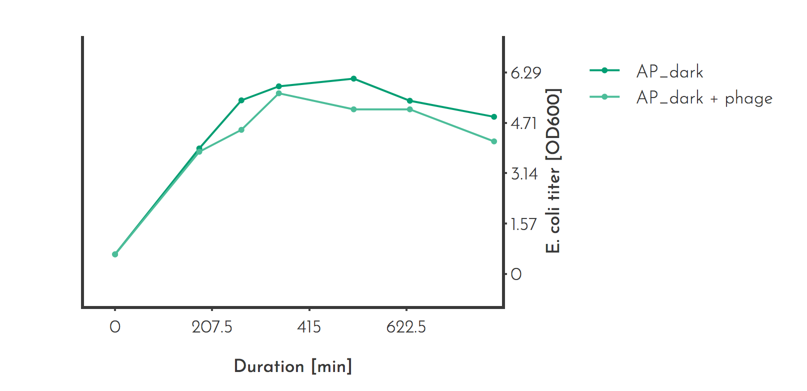
Figure 1: E. coli titer measurement for estimation of the E. coli capacity
The experiment was carried out in triplicates, the mean is plottet. If the optical density was higher than 1, samples were diluted and measured. The accessory plasmid (AP_dark) has a phage shock promotor under which gene III of the phage is expressed. The culture volume was 20 ml.
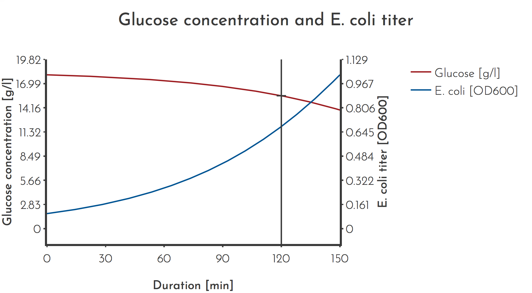
Figure 2: Modeled Glucose and E. coli titer for a representative PREDCEL experiment
Most PREDCEL experiments were carried out with a glucose concentration of \(c_{G_{M} } = 100 \: mmol/l\), an initial OD of \(c_{E} = 0.1\), usually phage was added at \(t = 120 \: min\).
Calculated with the Interactive Webtool of this model
Calculated with the Interactive Webtool of this model
Theory - Arabinose
An interactive webtool implementing the arabinose model described below is available.Arabinose functions as inducer for the mutagenesis plasmids, it is assumed to not be degraded by E. coli in this model. Thus in a PREDCEL experiment arabinose concentration \(c_{A}\) is constant over time, because neither the total volume changes nor the amount of arabinose in the flask. $$ \frac{\partial c_{A_{L} } }{\partial t} = 0 $$ and the concentration is the starting concentration: $$ c_{A_{L} }(t) = c_{A_{L} }(t_{0}) $$ If the arabinose concentration is modeled for a lagoon supplied by a turbidostat with a separate supply of arabinose solution, the system converges to a steady state, when turbidostat volume \(V_{T}\), arabinose influx \(\Phi_{S}\) and flow rate of turbidostat \(\Phi_{T}\) are constant. In that case $$ \frac{\partial c_{A} }{\partial t} = 0 $$ is true. The change in lagoon arabinose concentration \(c_{A_{L} }\) is described by $$ \frac{\partial c_{A_{L} }(t)}{\partial t} = \Phi_{S} \cdot c_{A_{S} } - \Phi_{L} \cdot c_{A_{L}(t)} $$ \(\Phi_{S}\) and \(\Phi_{L}\) are measured relative to the lagoon volume. The arabinose concentration in the lagoon \(c_{A_{L} }\) can then be calculated using the concentration of the arabinose solution with which the lagoon is supplied \(c_{A_{S} }\). $$ c_{A_{L} } = \frac{\Phi_{S} }{\Phi_{L} } \cdot c_{A_{S} } $$ However, in some cases it may be relevant to estimate when a given percentage of the equilibrium concentration is reached. To make statements about that, the differential equation is solved to $$ c_{A_{L} }(t) = \frac{\Phi_{S} }{\Phi_{L} } \cdot c_{A_{S} } - \big(\frac{\Phi_{S} }{\Phi_{L} } \cdot c_{A_{S} } - c_{A_{L} }(t_{0})\big) \cdot e^{-\Phi_{L} t} $$
Table 2: Variables and Parameters used for the calculation of the glucose and E. coli concentrations List of all paramters and variables used in the numeric solution of this model. Also have a look at the interactive webtool based on this model
| Symbol | Value and Unit | Explanation |
|---|---|---|
| \(c_{A_{L} }\) | [g/ml] | Arabinose concentration in Lagoon |
| \(c_{A_{L}(t_{0}) }\) | [g/ml] | Initial Arabinose concentration in Lagoon |
| \(\Phi_{S}\) | [lagoon volumes/h] | Flow rate of inducer supply relative to lagoon volume |
| \(\Phi_{L} \) | [lagoon volumes/h] | Flow rate of lagoon |
Practice - Arabinose
In all performed PACE experiments the inducer flow rate was \(\Phi_{S} = 2 ml/h \) and the lagoon volume was \(V_{L} = 100 ml\), resulting in a normalised \(Phi_{S} = 0.02\).In the first experiments, \(c_{A_{S} }\) was set to 50 g/l, corresponding to 333 mmol/l. The conditions result in \(c_{A_{L} } = 1 g/l\), or 6 mmol/l.
Later the inducer concentration was doubled to \(c_{A_{S} } = 100 g/l), resulting in a lagoon concentration of \(c_{A_{L} } = 2 g/l) or 12 mmol/l.
To circumvent low arabinose concentrations in the beginning, the experiment can be started with starting concentrations above the equilibrium concentration. Since no negative effects of high arabinose concentrations on the outcome of PACE
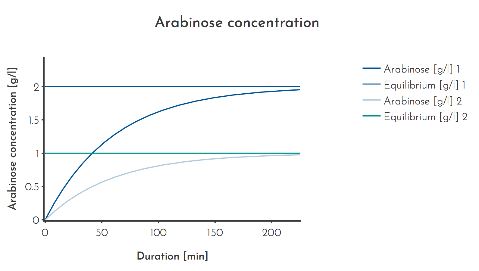
Figure 3: Arabinose concentrations used for PACE
Initially a lower inducer concentration was used (Plot 2), later it was doubled to 100 g/l. The prediction shows that it takes 3 h until 90 % of the equilibrium concentration is reached.
Calculated with the Interactive Webtool of this model
Calculated with the Interactive Webtool of this model
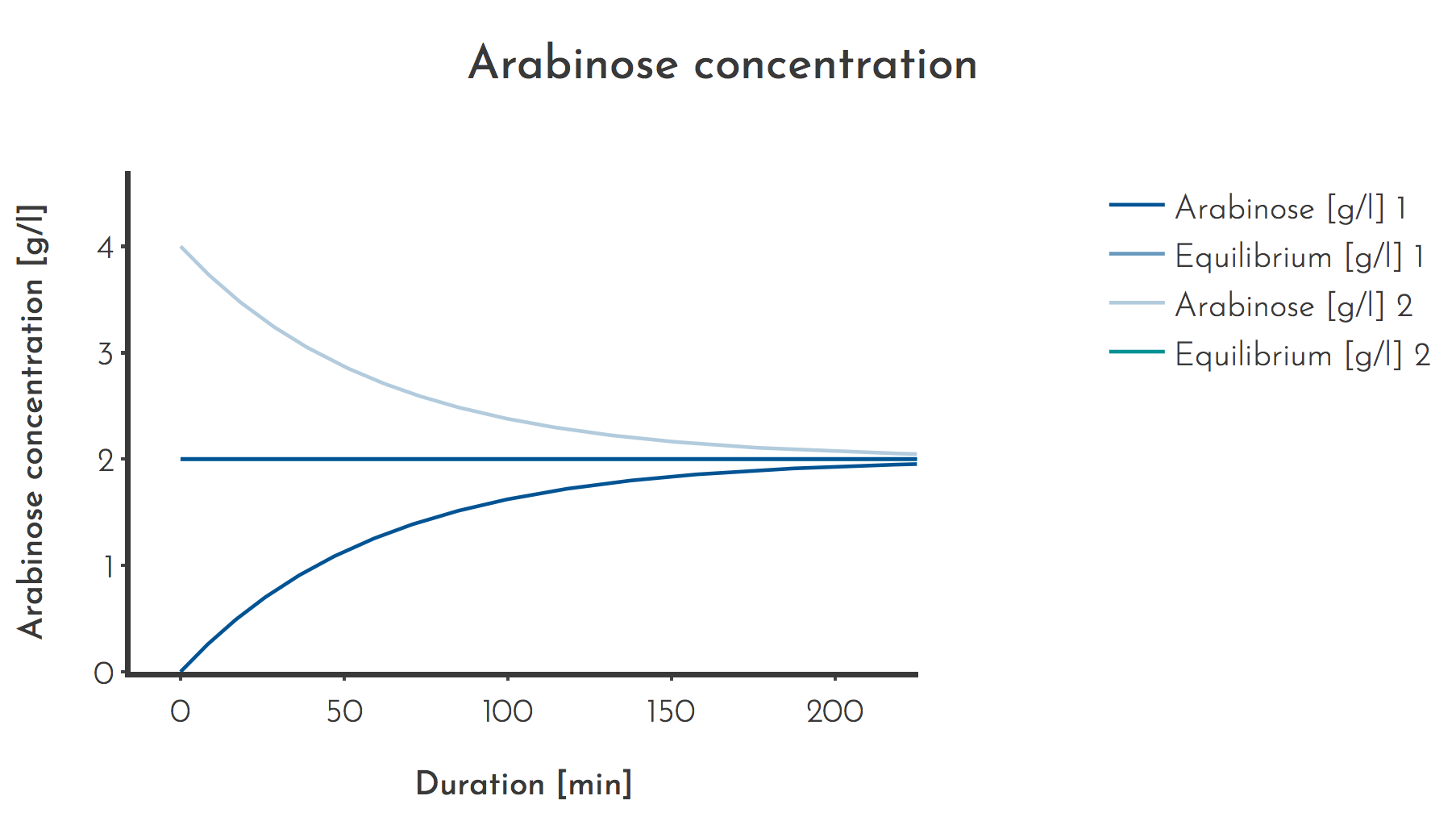
Figure 4: Effect of starting concentrations higher than the equilibrium concentrations
The Arabinose concentration approaches the equilibrium concentration from either above (Plot 1) or below (Plot 2). Assumed values are \(c_{A_{S} } = 100 \: g/l\), \(\Phi_{L} = 1 \) lagoon volumes/h, \(\Phi_{A} = 0.02\) lagoon volumes/h, \(t = 120 min \), \(c_{A_{L} } (t_{0}) = 0 g/l\) or \(c_{A_{L} }(t_{0}) 4 g/l\)
Calculated with the Interactive Webtool of this model
Calculated with the Interactive Webtool of this model
References