Team:HFLS H2Z Hangzhou/Model
Template loop detected: Template:HFLS H2Z Hangzhou<!DOCTYPE html>
Modeling
Overview
In the modeling part, we basically made two models. One is for predicting time required for nitrite decomposition by our enzyme, which could be used when applying our product to the industrial production. The second model is the mechanism of our software.
Quick Menu
Time Prediction
Software
A Model for Predicting Time Required to Decompose Nitrite
1 Abstract
As stated in the project breif, our ultimate goal is to reduce the time needed for $\ce{NO2-}$ to decompose. Therefore, the prediction of the time needed to reduce $\ce{NO2-}$ to a healthy level is a crucial part to apply our project to industrial production. We built three models for each of our enzymes based on enzyme kinetics to reach our final target.2 Model
2.1 Variables
We use the following symbols to represent the variables included in our model.| $C_s$ | Concentration of substrate($\ce{NO2–}$ in this case) |
| $C_p$ | Concentration of productCeConcentration of enzyme |
| $V_{max}$ | Maximum rate of reaction |
| $K_m$ | Michaelis-Menten constant |
| $K_c$ | A trivial constant in a solution for the differential equation |
| $K_{cat}$ | Turnover number |
| $c_n$ | Trivial constant |
2.2 Model for the Relation between ∆t and Cs
The rate of reaction of a enzymatic reaction can be modelled by the well-known Michaelis-Mentenequation, which is stated as $$ v = \frac{dC_p}{dt} = - \frac{dC_s}{dt} = \frac{V_{max} C_s}{K_m + C_s} $$ What we need to get to reach our goal is to find a function of $ C_s = f(t) $, so that we can predict the time spent, $ \Delta t $, by substituting the initial concentration $ C_{0} $ and the target concentration $ C_{t} $ to get the time difference.Therefore, by separating the variables in two sides of the equation and integrating both sides, we can get one solution set to this differential equation. $$ - \frac{dC_s}{dt} = \frac{V_{max} C_s}{K_m + C_s} $$ $$ - \frac{K_m + C_s}{V_{max} C_s} dC_s = dt $$ $$ - \int \frac{K_m + C_s}{V_{max} C_s} dC_s = \int dt $$ $$ - \int \frac{K_m}{V_{max}} \frac{1}{C_s} + \frac{1}{V_{max}} dC_s = t + c_1 $$ $$ - \frac{K_m}{V_{max}} ln(C_s) - \frac{1}{V_{max}} C_s + c_2 = t + c_1 $$ $$ - \frac{K_m}{V_{max}} ln(C_s) - \frac{1}{V_{max}} C_s + (c_2 - c_1) = t $$ Let $ K_{c} = c_2 - c_1 $, we get our final solution $$ t = - \frac{K_m}{V_{max}} ln(C_s) - \frac{1}{V_{max}} C_s + K_{c} $$ Where $ K_m $ and $ V_{max} $ can be found through our experiments stated below.
So to use the model, we simply need to substitute $ C_s = C_0 $, $ t = 0 $ to the solution, and get $$ K_c = \frac{K_m}{V_{max}} ln(C_0) + \frac{1}{V_{max}} C_0 $$ And substitute $ K_c $ back, we get $$ \Delta t = t - 0 = \frac{K_m}{V_{max}} (ln(C_0) - ln(C_s)) + \frac{1}{V_{max}} (C_0 - C_s) $$ $$ \Delta t = \frac{K_m}{V_{max}} (ln(C_0 / C_s)) + \frac{1}{V_{max}} (C_0 - C_s) $$ And $ C_s $ is our target concentration of substrate($\ce{NO2-}$).
Because $ V_{max} $ and enzyme concentration $ C_e $ are related by the turnover number $ K_{cat} $ $$ V_{max} = K_{cat} C_e $$ We can rewrite the equation as $$ \Delta t = \frac{K_m}{K_{cat} C_e} (ln(C_0 / C_s)) + \frac{1}{K_{cat} C_e} (C_0 - C_s) $$ $$ \Delta t = \frac{K_m (ln(C_0 / C_s)) + (C_0 - C_s)}{K_{cat} C_e} $$
2.3 Determine the Parameters
The last step completing this model is to determine $ K_m $ and $ V_{max} $ in this model. We used the Lineweaver-Burk plot to find the two constants.By taking the reciprocals of two sides the Michaelis-Menten equation, we can get a linear relation between $ \frac{1}{v} $ and $ \frac{1}{C_s} $, which then can be used to determine the parameters $ K_m $ and $ V_{max} $. $$ - \frac{1}{\frac{dC_s}{dt}} = \frac{K_m + C_s}{V_{max} C_s} $$ $$ - \frac{1}{\frac{dC_s}{dt}} = \frac{K_m}{V_{max}} \frac{1}{C_s} + \frac{1}{V_{max}} $$ So by linear regression of our experiment data($ - \frac{1}{\frac{dC_s}{dt}} $ against $ \frac{1}{C_s} $), we computed the parameters(Figure 2.3.1).
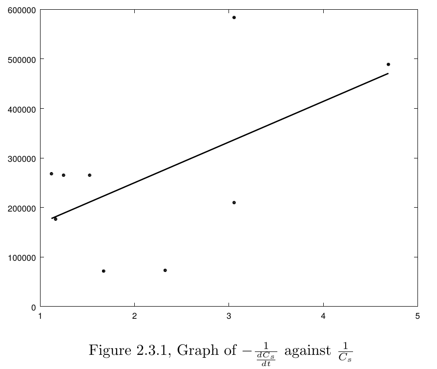 The regression results are
| $K_m$ | 0.95489 $ mmol\ dm^{-3} $ |
| $V_{max}$ | 1.1637e-05 $ mmol\ dm^{-3}\ s^{-1} $ |
Substituting back the parameters, we get the $ C_s $-$ t $ graph(the dots are our data from the experiments)

2.4 Model simulation in MATLAB
%%%%%%%%%%%%% data %%%%%%%%%%%%%

% absorbance
A = [ 0.408 0.393 0.367 0.302 0.276 0.201 0.155 0.155 0.104 ];
t = [ 3 5.5 7.5 20.5 22.5 25 28 31 46.5 ]; % in hours

% parameters of the standard curve(absorbance against concentration of NaNO2 in mg/L)
std_k = 0.647659;
std_b = 0.00872129;

%%%%%%%%%%%%% model %%%%%%%%%%%%%

% convert hr to sec
t = t .* (60 * 60);

% times 100 because solution is diluted
C = (A .- std_b) ./ std_k ./ (23 + 14 + 32) .* 100;
C0 = C(1);

v = -gradient(C) ./ gradient(t);
ln = @(x) log(x) ./ log(e);

poly = polyfit(1 ./ C, 1 ./ v, 1);

km = poly(1) / poly(2) % in mmol/L
vmax = 1 / poly(2) % in mmol/L/s

% model equation
m1 = @(cs) (km .* (ln(C0 ./ cs)) .+ (C0 .- cs)) ./ vmax;

plot(t, C, '.k'); hold;
plot(m1(linspace(0, C0, 100)), linspace(0, C0, 100), 'k');

ylabel('Cs');
xlabel('t/s');
2.5 Further Improvement
Although we can get the basic relation between concentration of $\ce{NO2-}$ and time, there are still some factors we haven't considered. Firstly, the relation between enzyme concentration and cell concentration is still not clear. So in a real situation, where the bacteria are put into the pickle mixutre, the increase in the concentration of our enzyme is not included in our model. We hope that our future improvement of the model will allow us to more effectively predict the time required in a real production situation.3 Reference
1 |
J K Kristjansson and T C Hollocher, "First practical assay for soluble nitrous oxide reductase of denitrifying bacteria and a partial kinetic characterization". J. Biol. Chem. 1980, 255:704-707. |
2 |
Lineweaver, H; Burk, D. (1934). "The determination of enzyme dissociation constants". Journal of the American Chemical Society. 56 (3): 658–666. doi:10.1021/ja01318a036. |
3 |
Michaelis, L.; Menten, M.L. (1913). "Die Kinetik der Invertinwirkung". Biochem Z. 49: 333–369 (recent translation, and an older partial translation) |
Software
When we talk about processing the data, basically, it means to study the pattern behind existing datasets. One common practice is to use statistic method to display the datasets on a table, and then form a curve across all valid data. If the curve perfectly cuts through the dataset, it is referred to as best-fit. The significance behind best-fit line is to reveal the relationship between independent variable and dependent variable, which makes a great contribution to people's life.The first step to perform a regression is to form a feature space. Dimensions of a feature space depends on the scale of your dataset. For example, if you have twenty-six groups of data, you form a twenty-six dimensional feature space. Traditionally, biologists modify the best-fit line by narrowing down the variance, which is a typical kind of linear regression.
Today, with the advent of AI, biologists have more choices of data processing. One of the popular models is neural networks based on back propagation, and the other one is machine learning based logistic regression. From a high school IGEM participant's scope, team HFLS_H2Z will show you the difference between these models and the scope of their abilities.
Neural networks VS Linear regression
Judging from the outcome, the difference between linear regression and the neural network based on back propagation is their accuracy of estimates.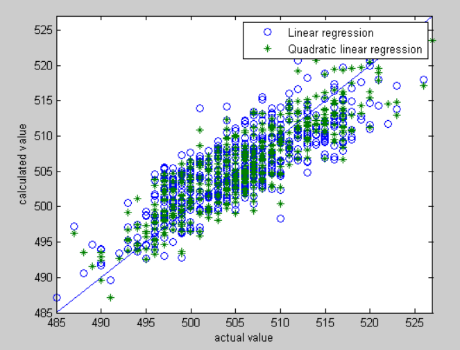
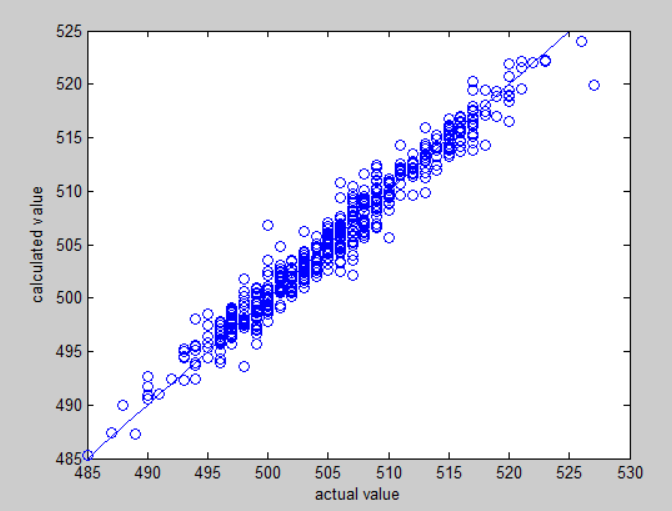 Clearly, we can see that neural network perform better than linear regression on fitting. The secret behind neural network's accuracy is attributed to back propagation, the mechanism constantly modify the net.
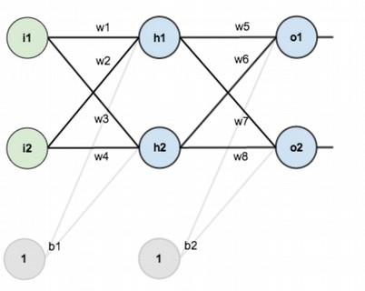 Neural networks consist of neurons, and we divide neurons into three layers: the first one is input layer, the second one is hidden layer, and the third one is output layer.
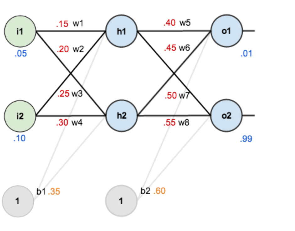 To build a net, we set initial values to each weight. Based on linear regression equation, we perform a forward propagation. Take input1 as an example,
$$ net_{h1} = w_1 \times i_1 + w_2 \times i_2 + b_1 \times 1 $$
$$ net_{h1} = 0.15 \times 0.05 + 0.2 \times 0.1 + 0.35 \times 1 = 0.3775 $$
Clearly, we can see there is a huge difference between calculated output1 (0.593269992) and actual value (0.01). At this point, we need to perform a back propagation to modify each weight.
To build a net, we set initial values to each weight. Based on linear regression equation, we perform a forward propagation. Take input1 as an example,
$$ net_{h1} = w_1 \times i_1 + w_2 \times i_2 + b_1 \times 1 $$
$$ net_{h1} = 0.15 \times 0.05 + 0.2 \times 0.1 + 0.35 \times 1 = 0.3775 $$
Clearly, we can see there is a huge difference between calculated output1 (0.593269992) and actual value (0.01). At this point, we need to perform a back propagation to modify each weight.
 First, we calculate the square error.
$$ E_{total} = \sum \frac{1}{2} (\mbox{target} - \mbox{output})^2 = E_1 + E_2 = 0.274811083 + 0.023560026 = 0.298371109 $$
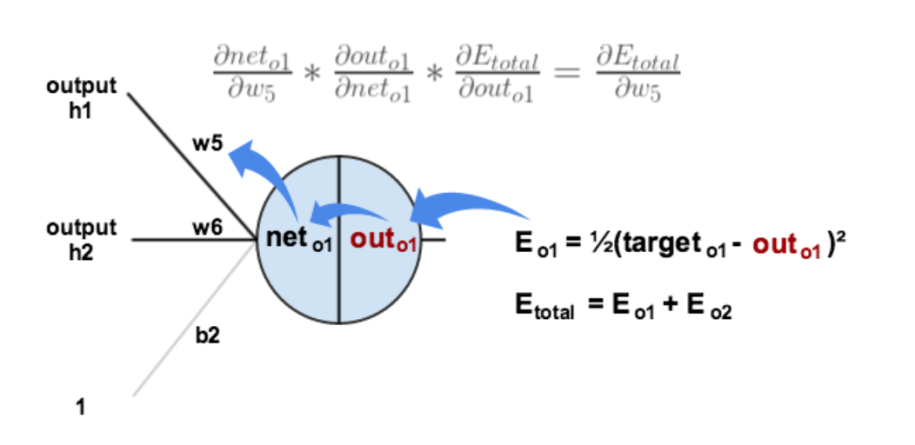
We hope we can find out how each weight influence the outcome. Take w5 as an example, we use chain rule to figure out its partial derivative, which reflects how influence the total square error.
$$ \frac{\delta E_{total}}{\delta w_5} = \frac{\delta E_{total}}{\delta \mbox{out}_{o1}} \times \frac{\delta \mbox{out}_{o1}}{\delta \mbox{net}_{o1}} \times \frac{\delta \mbox{net}_{o1}}{\delta w_5} = 0.74136507 \times 0.186815602 \times 0.593269992 = 0.082167041 $$
And it enables us to update the value of $ w_5 $. $ \eta $ represents the study rate of the net.
$$ w_{5_new} = w_5 - \eta \times \frac{\delta E_{total}}{\delta w_5} = 0.4 - 0.5 \times 0.082167041 = 0.3591648 $$
The back propagation constantly modifies the value of each weight. It ensures that the eventual net will be the best-fit one for the dataset. And this is why it performs better than linear regression. On the contrast, linear regression is more about forward propagation.
First, we calculate the square error.
$$ E_{total} = \sum \frac{1}{2} (\mbox{target} - \mbox{output})^2 = E_1 + E_2 = 0.274811083 + 0.023560026 = 0.298371109 $$
We hope we can find out how each weight influence the outcome. Take w5 as an example, we use chain rule to figure out its partial derivative, which reflects how influence the total square error.
$$ \frac{\delta E_{total}}{\delta w_5} = \frac{\delta E_{total}}{\delta \mbox{out}_{o1}} \times \frac{\delta \mbox{out}_{o1}}{\delta \mbox{net}_{o1}} \times \frac{\delta \mbox{net}_{o1}}{\delta w_5} = 0.74136507 \times 0.186815602 \times 0.593269992 = 0.082167041 $$
And it enables us to update the value of $ w_5 $. $ \eta $ represents the study rate of the net.
$$ w_{5_new} = w_5 - \eta \times \frac{\delta E_{total}}{\delta w_5} = 0.4 - 0.5 \times 0.082167041 = 0.3591648 $$
The back propagation constantly modifies the value of each weight. It ensures that the eventual net will be the best-fit one for the dataset. And this is why it performs better than linear regression. On the contrast, linear regression is more about forward propagation.
But it does not mean that neural network definitely performs better than linear regression. First, it costs time to train a net. Second, the net requires large datasets. Third, it is difficult for high school beginners to create their own net. But we can say for certain that neural networks are strong tools to study the pattern behind data.
Logistic regression VS Linear regression
Logistic regression is appropriate for cases that data are binary dependent variables. For example, the output can take only two values, "0" and "1", which represent outcomes such as pass/fail, win/lose, alive/dead or healthy/sick. In comparison to linear regression, logistic regression is not sensitive to XXX. For example, according to the size of a tumor, doctors judge whether the tumor is malignant. The table 1.a and 1.b use linear regression. (Picture by Andrew Ng)
1 |
Zhang S, Zhang L, Qiu K, et al. Variable Selection in Logistic Regression Model[J]. Chinese Journal of Electronics, 2015, 24(4):813-817. |
2 |
Marla, Maniquiz, Soyoung, et al. Multiple linear regression models of urban runoff pollutant load and event mean concentration considering rainfall variables[J]. 环境科学学报(英文版), 2010, 22(6):946. |
3 |
Ng A. Efficient L1 Regularized Logistic Regression[J]. In AAAI-06, 2006, 1:1--9. |